This is an example of a structure determination by the method of Multiwavelength Anomalous Dispersion (MAD). This particular case is relatively straightfoward, but might serve as an introduction to the concepts and considerations involved.
This is v0.2 of the Example, last revised Feb 2006 by Phil Jeffrey
It proved fairly straightforward to grow SeMet crystals from conditions closely related to the native crystal conditions. Streak seeding helped too - one can grow SeMet xtals from native seeds and vice versa.
Anomalous scattering changes the atomic scattering factor for the atoms in question. The atomic scattering factor - typically called f(S) - is a real quantity that falls off in a gaussian-type way with resolution (i.e. |S|):
and is usually wavelength-independent. However in the case of anomalous scattering it is changed to:
where f0(S) is the usual energy-independent value (i.e. away from the absorption edge). Note that the f' and f'' components do not fall off with resolution unlike the atomic scattering factor. The symbol "S" refers to the diffraction vector whose length is characteristic of resolution (actually 1/d). The values of f' and f'' can be looked up in tables, or it is better if you extract them from your own empirical fluorescence scan using a program like CHOOCH:
Depending on how much of a purist you are, there are quite a number of ways to collect MAD data. All ways require you to collect at least three datasets at different energies, so every MAD data collection is at least 3 times longer than a typical native dataset. In addition, because anomalous scattering violates Friedel's Law, the reflections (h,k,l) and (-h,-k,-l) have different intensities. In fact it's this difference that is the so-called anomalous difference. This loss of symmetry in the diffraction pattern means that your average redundancy (i.e. the ratio between the number of observations and the number of symmetry-merged reflections) will go down, which means that people often end up collecting twice as much data per wavelength than you would do in a native dataset.
If you're collecting 6x the amount of data as you would for a native dataset, radiation damage becomes a huge factor. At the very least you need to cut your exposure time per frame down by a factor of six compared to a dataset in which you started to observe radiation damage. There's some evidence that you should cut it down even further than that, since the anomalous scatterers suffer radiation damage faster than the rest of the crystal.
Since you reduce your exposure by a factor of 6, Poisson (counting) statistics suggest that your signal/noise ratio is going to drop by SQRT(6), or about 2.4x. This is not good news since your expected anomalous scattering signal is usually quite small. We can estimate the signal using this form and the expected number of scatterers. Our protein contains 5 methionine, but one of them is the N-terminal Met so that's usually disordered. Assuming 4 Met for 190 residues we get an estimated signal of 5% at resolutions lower than 3 Å in the most optimistic scenario assuming they are ordered and completely substituted. One SeMet per nearly 50 amino acids is in the acceptable range for MAD experiments for good diffractors. One per 100 is toward the upper limit of what is practical for MAD experiments since the signal is a very small number compared to typical data accuracy. In order to measure our MAD data acceptably, the Rsymm needs to be <5% in the resolution shells we are interested in.
Take a look at the SCALEPACK log file for your native data - just how far is that usable anomalous signal going to go ?
OK, now let's also look at the bright side and notice that the relative magnitude of the anomalous signal increases with resolution so that if your crystals diffract well you can measure the anomalous differences rather well at moderate to high resolutions. Unfortunately most MAD structure determinations that I've done have had usable MAD phases to about 3 Å and no further. C'est la vie.
You'll probably need to do a fluorescence scan (which measures f'' anomalous scattering from your crystal, and f' can be calculated from f'' using the Kramers-Kronig equation) to verify the presence and location of the absorption edge for the crystal. You can use experience-derived wavelengths/energies for MAD data collection, but you should do this only as a last resort since it relies on the beamline to be well-calibrated. You also need to use a beamline with good energy resolution since the difference in energy between the peak (max f'') and inflection (min f') is often only a few eV out of 10,000 eV. If you analyze the fluoresence scan with Chooch it will give you the recommended wavelengths, and estimates for f'' and f', but if not:
This is the Se edge plotted by edgeplots:
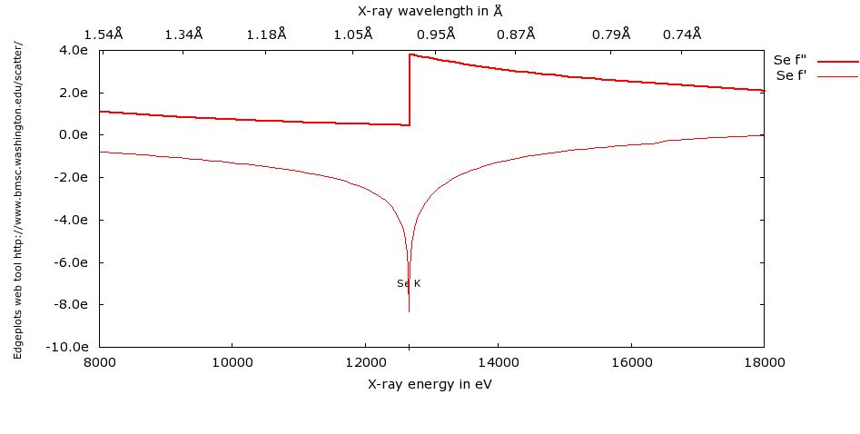
The importance of doing your own fluoresence scans on your own crystal is emphasized by the page on theory vs. reality - look at the plot and notice how the theoretical and experimental edge locations differ so your peak and inflection wavelengths from a theoretical plot would be completely wrong. The high energy remote would be OK. These differences occur because of changes in the chemical environment of the element with respect to the prediction for the isolated element or ion.
There's no substitute for doing your own fluorescence scan, but if it doesn't work for you (low signal or other issues) these values have historically worked quite well for me:
| Element | eV | λ Å | eV | λ Å | eV | λ Å | ||||||
|---|---|---|---|---|---|---|---|---|---|---|---|---|
| Se | Inflection | 12660 | 0.979 | Peak | 12662 | 0.979 | Remote | 12860 | 0.964 | |||
| Hg | Inflection | 12286 | 1.009 | Peak | 12320 | 1.006 | Remote | 12540 | 0.996 | |||
| Au | Inflection | 11927 | 1.039 | Peak | 11932 | 1.039 | Remote | 12230 | 1.014 | |||
| Pt | Inflection | 11567 | 1.072 | Peak | 11572 | 1.071 | Remote | 11867 | 1.045 | |||
| Zn | Inflection | 9664 | 1.283 | Peak | 9671 | 1.282 | Remote | 9824 | 1.262 |
In fact I have collected Zn MAD data based on the above wavelengths alone, where the fluorescence scan was unclear. Additionally, the Hg edge is so broad you might as well use the above wavelengths (the f' minimum is shallow and broad and there is no clear f'' peak).
Now we need to actually collect the data. Exposure time is set by the amount of data you want to collect while reducing radiation damage to the bare minimum. What's left is strategy and starting point. The traditional purist method is to do the inverse beam strategy while cycling through the three wavelengths, with the dataset(s) broken up into wedges, something like this:
| Start | Wedge | Energy |
|---|---|---|
| Phi=0° | 0-20° | Inflection |
| Phi=180° | 180-200° | Inflection |
| Phi=0° | 0-20° | Peak |
| Phi=180° | 180-200° | Peak |
| Phi=0° | 0-20° | Remote |
| Phi=180° | 180-200° | Remote |
| Phi=20° | 20-40° | Inflection |
| Phi=200° | 200-220° | Inflection |
| Phi=20° | 20-40° | Peak |
| Phi=200° | 200-220° | Peak |
| etc |
where inverse beam means recording small data wedges at phi and phi+180°. (The starting point of 0° is just an arbitrary choice for this example). The idea behind inverse beam is that you record reflections (h,k,l) and (-h,-k,-l) close together in time for specific reflections, with approximately the same absorption behavior. However in practice most of the power of inverse beam is lost if you just lump all these wedges together in one scaling run where symmetry-related reflections from multiple wedges get averaged. So it's a waste of time doing it. Also, the problem with shuffling through the wavelengths is that any given wavelength is only complete right at the end of the dataset, so if there's a power outage, or your crystal dies in the beam, or your crystal ices up, you've got 3 incomplete datasets. There's also overhead (in time) every time you change wedge or wavelength. How much overhead varies from beamline to beamline. The upside of doing inverse beam is that your redundancy gets doubled, and this is often a very good thing.
My preferred strategy is a modified streamlined inverse beam, roughly as follows (in this example for 90 degrees of data):
| Start | Wedge | Energy |
|---|---|---|
| Phi=0° | 0-30° | Peak |
| Phi=180° | 180-210° | Peak |
| Phi=30° | 30-60° | Peak |
| Phi=210° | 210-240° | Peak |
| Phi=60° | 60-90° | Peak |
| Phi=210° | 240-270° | Peak |
| Phi=0° | 0-30° | Remote |
| Phi=180° | 180-210° | Remote |
| Phi=30° | 30-60° | Remote |
| Phi=210° | 210-240° | Remote |
| Phi=60° | 60-90° | Remote |
| Phi=210° | 240-270° | Remote |
| Phi=0° | 0-30° | Inflection |
| Phi=180° | 180-210° | Inflection |
| Phi=30° | 30-60° | Inflection |
| Phi=210° | 210-240° | Inflection |
| Phi=60° | 60-90° | Inflection |
| Phi=210° | 240-270° | Inflection |
This has thicker wedges (30 vs 20 °) and collects entire datasets first. The idea is that if all else fails, you can try and do SAD (single wavelength) instead of MAD. Also I personally value Peak and Remote over Inflection because Peak and Remote have the highest values of f'' and this seems to give the most phasing power in my own hands (compared to the f' contribution). The program SHARP seems to do a little better extracting a useful phasing signal out of the f' contribution, however. Strategies have to be modified for real-world situations - e.g. at CHESS where the beam refills every 70 minutes, you don't want to split the Peak or Inflection data collections across a fill because they are very sensitive to precise energy and the energy may shift a little between fills. Remote is less sensitive to this so you may end up changing data collection order.
The starting point and total angular range depends on the orientation of the crystal and it's symmetry. P1 needs 170+ degrees, P21 needs 110-140 degrees, P212121 needs ~75 degrees, P41212 needs about 50 degrees, and so on. You should have a decent idea of how much data you will need to collect and where to start from based on your native data - this is usually reproducible from the same point with respect to crystal morphology, or you can use a data collection strategy prediction program like the one that's part of HKL2000.
For the sake of accuracy you should do fluorescence scans after every fill - note that many beamlines are not entirely stable for the first 10 minutes after the fill (e.g. F2, X25 etc) because the optics need to warm back up. Again note that MAD datasets are very intolerant to errors introduced during data collection and so you should take copious notes if you need to trace back the source of an error and process the data as you proceed.
ADD PARTIALS 1 TO 30, 31 TO 60, 61 TO 90You also want to check things like the variation in the scale factors and B-factors to make sure that they vary the expected amount during data collection, after consideration of beam intensity. Unexpected variations in scale factors can indicate severe problems with crystal centering which can otherwise hopelessly compromize your data quality. If you process as you collect the data, you can spot this sort of error in real time. Also if you restrain the scale factors and B-factors you need to make sure that these restraints are applied at the appropriate level and not across things like beam fills. Over-restraining these parameters can hurt scaling.
You must scale each different wavelength separately but you'll want to lump both sides of the inverse beam strategy for the same wavelength together. Remember to output the anomalous data using the ANOMALOUS keyword in SCALEPACK. Remember that the keyword ANOMALOUS still treats intensity of reflection (hkl) (henceforth I(+)) and the intensity of reflection (-h,-k,-l) (I(-)) as symmetry-related for the point of view of determining scale factors - this is not a bad approximation if the anomalous signal is low, as is typically the case. It does not merge I(+) and I(-) before output, however. But the anomalous signal will inflate Rsymm a little. The alternative, only if you have a great deal of redundancy is to use the keyword SCALE ANOMALOUS which treats I(+) and I(-) as completely independent throughout scaling.
If you have really low redundancy (e.g. you are collecting data in triclinic or monoclinic space groups) you can determine the per-frame scale factors and B-factors based on merging all the wavelengths together and then using these scale factors and B-factors to scale the individual wavelengths separately. Consult my page on data processing right at the end of the tutorial, for examples of SCALEPACK command files to do this.
You can also get a good initial idea of the usefulness of your anomalous data by looking at the signal/noise ratio and correlation between different energies of the anomalous signal (I(+)-I(-)). The program SHELXC is the one I favor for this because it runs very quickly and has a compact syntax:
shelxc se1 << EOF
HREM se1rm.sca
PEAK se1pk.sca
INFL se1in.sca
LREM se1lo.sca
CELL 35.104  63.496  76.458 90. 90. 90.
SPAG P212121
FIND 8
NTRY 50
EOF
where perhaps the only mysterious parameters are FIND (the number of sites to find) and NTRY (the number of attempts to make) which don't become relevent until you run SHELXD. Dataset HREM is the high energy remote and LREM is the low energy remote. I collected the latter largely so I could attempt to improve the resolution of the SeMet data I collected - yes, this data does go to 1.5 Å. Your data will not.
For the datasets collected, this is the output:
    52202 Reflections read from LREM file se1lo.sca
    28027 Unique reflections, highest resolution  1.499 Angstroms

 Resl.   Inf - 8.0 - 6.0 - 5.0 - 4.0 - 3.5 - 3.0 - 2.5 - 2.1 - 1.9 - 1.7 - 1.50
 N(data)     177   277   341   763   751  1327  2569  4183  3565  5412  8662
 <I/sig>    43.7  48.9  50.7  56.2  52.2  32.5  28.5  23.6  16.5  10.6   5.6
 %Complete  74.1  97.2  98.6  99.2  99.2  98.0  99.5  99.7  99.7  99.8  99.4
 <d"/sig>    .91  1.17  1.00   .99  1.22   .98  1.03   .97   .89   .77   .74

    32819 Reflections read from HREM file se1rm.sca
    17676 Unique reflections, highest resolution  1.749 Angstroms

 Resl.   Inf - 8.0 - 6.0 - 5.0 - 4.0 - 3.5 - 3.0 - 2.6 - 2.4 - 2.2 - 2.0 - 1.75
 N(data)     121   265   335   727   747  1344  1914  1465  2033  2939  5786
 <I/sig>    40.5  44.7  46.0  48.2  47.2  43.4  38.2  34.3  31.1  24.9  15.2
 %Complete  50.6  93.0  96.8  94.5  98.7  99.3  99.5  99.8  99.8  99.6  99.4
 <d"/sig>   2.66  3.16  2.60  2.12  1.98  1.95  1.93  1.86  1.74  1.58  1.31

    32790 Reflections read from PEAK file se1pk.sca
    17730 Unique reflections, highest resolution  1.749 Angstroms

 Resl.   Inf - 8.0 - 6.0 - 5.0 - 4.0 - 3.5 - 3.0 - 2.6 - 2.4 - 2.2 - 2.0 - 1.75
 N(data)     158   277   341   754   748  1346  1917  1466  2034  2936  5753
 <I/sig>    42.2  40.6  41.2  45.4  43.6  39.2  33.7  29.2  25.8  19.9  10.6
 %Complete  66.1  97.2  98.6  98.0  98.8  99.4  99.6  99.9  99.9  99.5  98.8
 <d"/sig>   2.71  3.08  2.89  2.35  2.06  2.09  2.13  2.00  1.82  1.58  1.31

    32721 Reflections read from INFL file se1in.sca
    17683 Unique reflections, highest resolution  1.750 Angstroms

 Resl.   Inf - 8.0 - 6.0 - 5.0 - 4.0 - 3.5 - 3.0 - 2.6 - 2.4 - 2.2 - 2.0 - 1.75
 N(data)     115   269   337   731   749  1347  1917  1466  2034  2938  5780
 <I/sig>    40.4  42.4  44.5  47.9  46.6  42.7  37.4  33.3  29.9  23.5  13.5
 %Complete  48.1  94.4  97.4  95.1  98.9  99.5  99.6  99.9  99.9  99.6  99.6
 <d"/sig>   2.97  3.30  3.06  2.40  2.14  2.12  2.13  2.03  1.85  1.67  1.40

 Correlation coefficients (%) between signed anomalous differences
 Resl.   Inf - 8.0 - 6.0 - 5.0 - 4.0 - 3.5 - 3.0 - 2.6 - 2.4 - 2.2 - 2.0 - 1.75
 LREM/HREM  69.4  74.7  57.8  35.3   -.9  25.0  25.0  21.5  21.8  18.2  17.1
 LREM/PEAK  49.0  64.7  48.1  34.0   3.0  24.3  23.0  16.7  25.2  25.0  20.5
 LREM/INFL  62.4  70.0  52.8  41.0   2.1  25.1  25.3  19.7  22.3  26.3  22.6
 HREM/PEAK  94.2  95.5  92.2  76.5  66.9  62.9  68.2  65.6  60.6  59.1  56.7
 HREM/INFL  94.7  94.2  91.1  80.9  75.8  67.7  71.7  69.3  64.5  64.8  60.9
 PEAK/INFL  96.8  95.8  96.7  86.3  78.1  78.8  81.8  79.2  74.3  71.0  66.9

 For zero signal <d'/sig> and <d"/sig> should be about 0.80
A couple of things make this almost ideal MAD data. First of all the d''/sig is relatively high over the entire resolution range - the data was measured well enough to get a decent anomalous signal (d'' = I(+) - I(-)). Compare the d''/sig for the peak dataset with that for the low energy remote (LREM), for example - we don't expect much d'' for LREM since it is on the low energy side of the absorption edge. Secondly, further evidence for data quality is the degree of correlation between the anomalous signals for separate datasets, which is >55% for HREM and PEAK over the entire resolution range. Cutoff values for usefulness for d''/sig is about 0.8, and that for correlation is about 30% so we're well above that.
We've collected pretty good MAD data - those of you with sharp eyes will detect that the INFL (inflection) dataset probably wasn't collected quite at the right location, since it has a d''/sig signal as good as PEAK over the entire range and the correlation between PEAK and INFL is the highest one.
Nevertheless this is truly excellent MAD data.
The simplest and tedious way is to calculate an anomalous difference Patterson, find the peaks on the Harker sections and calculate the relationship between the Harker peaks and the real space locations of the heavy atoms (Se, in this case). This is in fact how most of the MIR structures were done before the days of more reliable programs that automate this task.
More recently, the programs SOLVE and SHELX have supplied us with powerful tools that can quite predictably locate heavy atoms from anomalous or isomorphous data. Many peopls use SOLVE but I prefer SHELX since it is substantially faster (and I've used it more often). Assuming you've run the SHELXC example above, then SHELXC writes a command file that can be used by SHELXD, and all you need to do is type:
shelxd se1_faand the program will run. It actually takes a little while since we have told it to run for 50 cycles. SHELXD uses the data prepared by SHELXC, which includes a modification of the MAD data to reduce systematic errors in the MAD data (in the same way that the program REVISE does in CCP4 - see the online CCP4 documentation). Note that in changing wavelengths we alter the scaling of the anomalous signal - but the differences should in fact be the same except scaled by the magnitude of f''. This makes it possible to effectively "average" the anomalous signal for each reflection between different datasets to improve it's accuracy.
SHELXD is an example of a Direct Methods program that is routinely used to solve small molecule crystal structures (at very high resolutions) that has been adapted so that it can solve heavy atom substructures at much more modest resolutions (one might note that the number of reflections per atom are not dissimilar in these two situations). Direct Methods sometimes strikes people as being rather mystical but is based on a simple set of probablistic relationships like:
for a set of three strong reflections. SHELXD will generate multiple possible sets of phases for reflections related by these triplet phase invariants and analogous relationships and then improve and expand the phase estimates using the Tangent Formula. Each set of phases is then used to phased a heavy atom difference map (anomalous difference in the case of MAD, isomorphous difference from the case of MIR) whose peaks one might hope correspond to the heavy atom locations. It's self-evident that they often do in the case of good MAD data, or I wouldn't be using the program.
The correlation between the calculated and measured anomalous differences is a good way to get an idea of how each potential solution is. In this case the best one is 45% for all data and 37% for weak data, and this is a hallmark of a good solution - a good correlation on the weak data as well as just the strong ones. In fact the MAD data is so good, in effect all the solutions are more-or-less the same - typically you'll see a few good solutions and a bunch of incorrect ones. From looking at the result (in se1_fa.res) you can see that SHELXD finds four sites (the fourth column of numbers is the relative occupancy):
REM TRY     39   CC 45.18   CC(weak) 36.92   TIME      72 SECS
REM
TITL se1_fa.ins MAD in P212121
CELL    0.98    35.10   63.50   76.46  90.000  90.000  90.000
LATT  -1
SYMM 1/2-X, -Y, 1/2+Z
SYMM -X, 1/2+Y, 1/2-Z
SYMM 1/2+X, 1/2-Y, -Z
SFAC SE
UNIT   128
SE01   1   .143585   .537376   .012369   1.0000  0.2
SE02   1   .315178   .447250  -.061058    .9841  0.2
SE03   1   .583473   .543518   .094421    .8140  0.2
SE04   1   .881943   .546371   .213310    .6366  0.2
SE05   1   .704750   .563721   .276031    .1556  0.2
SE06   1   .555199   .442657   .134171    .1477  0.2
SE07   1   .754143   .612366  -.039116    .1452  0.2
SE08   1   .735634   .782303   .217743    .1281  0.2
SE09   1   .322693   .450851  -.131317    .0876  0.2
SE10   1   .868706   .582130   .035431    .0804  0.2
SE11   1   .681496   .260635   .060143    .0427  0.2
HKLF 3
END
Now that SHELXD has found the heavy atom sites, you can use these heavy atom sites in any other program to phase the MAD data - I continue to use SHELXE for phasing and solvent flattening. SOLVE does a better job with solvent flattening than SHELXE but is substantially slower. The program SHARP is the ultimate heavy atom phasing program, and will produce substantially better electron density maps than either SHELXE or SOLVE. Correspondingly it takes a long time to run, so it's mostly a question of how much patience you have vs. how much extra phasing power you need. In the case of this first example, the maps are good enough that we need nothing more powerful than SHELXE. In many other cases you can use a variety of approaches at a variety of stages to start off with halfway usable phases and then slowly improve upon them.
If you're a data purist, I strongly recommend using SHARP for all MAD and MIR phasing.
If you're a pragmatist, and "good enough" is what counts, then you use the program that gets an acceptable result the quickest. In this particular case I used SHELXE to do my phasing and solvent flattening. SHELXE is fast, has limited user intervention, and with good MAD data and correct heavy atom sites it will provide a decent MAD map. It will not produce the optimal map because Black Box programs rarely do that. In the case of another mystery structure, SHELXE produced an interpretable map but SHARP produced a much better map from the same sites and same data which then could be autobuilt using ARP/wARP saving a great deal of effort.
Solvent Flattening, a procedure originally pioneered by B.C. Wang, improves phases by the use of the additional information that the solvent regions are generally flat and featureless (hence the term "bulk solvent"). If one has a halfway decent set of phases, it's possible to find the solvent boundary by methods that look at volume-averaged electron density variation and/or height. There are various different algorithms to find the boundary but the basic idea is that the solvent is smoothed to it's mean electron density value, the map is fourier inverted (electron density -> structure factors) and the resultant modified phase values are combined with the experimental phase information via a weighting scheme that we won't go into. Typically an iterative procedure, the idea is that the experimental phases are modified slowly to drift toward and electron density map that is superior because it contains more information than the original experimental phases did. Of course, if you pick the solvent boundary incorrectly it will contain less phase information. If your phases are basically garbage to start off with, it's not going to help.
SOLVE/RESOLVE now has one that works at modest resolutions, but my personal favorite is the program ARP/wARP. wARP basically puts "free atoms" in positive peaks in the electron density map (or difference maps) and removes them from negative peaks, iteratively refining the structure and recalculating maps phased from that structure. In favorable cases these non-interacting "atoms" actually correspond to atom locations within your protein structure. If you get enough atoms in the right locations, wARP can interpret their locations in terms of a polypeptide backbone. If you give it the sequence, it will try and dock the sequence into the built backbone too.
In the best case scenario it will take your MAD map, refine the "free atom" locations and then autobuild your structure. It will usually miss flexible loops and mess up in metal-binding or cofactor sites, but since I autobuilt most of this structure on my Mac G5 at home while I was sleeping after getting back from the synchrotron trip, I think this is a pretty good deal, especially since this is only the second time I've ever managed to solve a structure at the synchrotron.