This guide is aimed at the mid-level - I don't provide derivations since they can be found elsewhere, I omit certain arcane details for the sake of brevity (e.g. the G-function is not discussed) but by the same token there isn't enough time or space to talk about basic crystallographic theory. There's a more advanced discussion of molecular replacement theory written by Dima Chirgadze if you have an interest in a more thorough explanation.
Last updated May 2010 with content and html code changes.
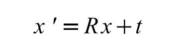
MR is fundamentally a six-dimensional problem:
where the coordinates of the "unknown" to be solved (x') are a simple transformation of the input model (x). Three parameters define a 3x3 rotation matrix (R) and three parameters define the translation vector (T). (x and x' are position vectors for each atom in the structure).
Because of the size of our models and the size of space to be searched, doing the six-dimensional search is a very time consuming process. For example, for a typical unit cell (orthorhombic, 100x100x100 Angstroms) this 6-D search sampled in a fairly coarse grid (5 degree rotation increments, 1 Ångstrom translation increments) has 36x36x18x50x50x50 = 3x10⁹ points. Even if each point took 1/100 second to evaluate, that would still be 8100 hours of computation. Computers have got faster, but only to a point.
The MR method was first developed in the 1960's, when computing power was negligable, so the method focussed on two much smaller 3-D searches: the Rotation Function (RFn), which determines the rotation matrix only; the Translation Function (TFn), which determines the translation vector given a rotation matrix. Even today, most MR programs use this "divide and conquer" approach because the sheer size of a six-dimensional search still makes it not the first choice.
Fractional coordinates express positions as fractions of a cell edge, in a coordinate system that is not necessarily orthogonal (example: PHASER and AMORE's translation function). Any set of coordinates can be mapped into the range 0...1 on each fractional axis since 0 and 1 are the vertices of the unit cell. Axial coordinates, although rarely used, express positions in Ångstroms along a cell edge (example: BRUTE's translation function). To convert axial to fractional just divide by the respective unit cell edge lengths. Cartesian coordinates are used frequently, and are expressed in Ångstroms in a standard orthogonal reference frame. This is the coordinate system that PDB files are in. However the way that the reference frame maps to the unit cell can potentially have several different definitions.
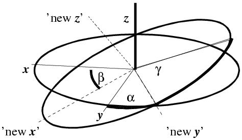
There are also a variety of ways to construct the rotation matrix, but in three dimensions you need at least three parameters. All rotation functions use a set of three angles (although there are other ways to define such a matrix). There are three major angle systems:
These angle systems are incompatible with each other - don't mix and match them ! However all the angle systems define a 3x3 rotation matrix.
For the sake of completeness: α, β, γ (alpha, beta, gamma) are the Eulerian angles for rotating axes as defined by Tony Crowther (Crowther (1972). The Molecular Replacement Method, edited by M.G. Rossmann, pp. 173-183. New York: Gordon & Breach). They rotate the model by rotating first through α about Z, then through β about the new Y, then through γ about the new Z. AMORE, ALMN and PHASER use this convention, amongst others. θ1, θ2, θ3 (theta1, theta2, theta3) is an older convention for angles, rotating first through θ1 about Z, then through θ2 about the new X, then through θ3 about the new Z. CNS and X-PLOR use this convention. You can perhaps see from the angle definitions that β = 0.0 and β = 180.0 are special positions in these angles systems where α and γ are redundant with each other. This also applies for θ2 =0 or =180. Peaks near these "special positions" tend to be smeared out because of this behavior. Sometimes you might also see θ+, θ2, θ-, which is a special case: θ+ = θ1 + θ3; θ- = θ1 - θ3. This system is constructed to deal with the redundancy at θ2=0 and θ2=180.
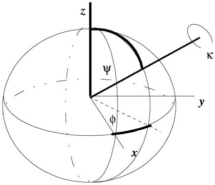
Only with the polar angle system is the degree of rotation in the matrix obvious (κ). Unfortunately the polar angles are often called different things: (φ, ψ, χ) or (φ, ω, κ) etc. The definition I encounter the most frequently is: κ is the rotation around the rotation axis, and φ and ψ define the direction of the axis. Psi (ψ) is the angle the rotation axis makes with the z axis. Phi (φ) is the angle that the axis makes with the x axis when the rotation axis is projected into the x/y plane. Kappa (κ) is the actual rotation about the axis. This is actually easy to compute from direction cosines if you normalise the length of the rotation axis. The original recasting of the Crowther rotation function into polar angles was by Tanaka (Acta Cryst. (1977). A33, 191-193).
Note also, for rotation matrices in Cartesian space that don't change the shape of the molecule:
Once you get out of Cartesian space and e.g. into axial or fractional systems all bets are off, but the nature of Cartesian space is that the metric for distance in any direction is the same which puts some constraints on rotation matrices.
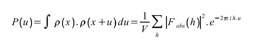
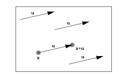
U is a vector in Patterson space. Rho (ρ) is the electron density at points (x) and (x+u). ERRATUM: there's an error in this equation, since the summation needs to be done over x (i.e. dx) not u. Patterson unit cells are the same size as the original crystallographic unit cell. However the vector u (Patterson space) is not the same as the vector x (unit cell space) although sometimes they are conflated. The conventional interpretation of the Patterson function is that it is consists of the weighted sum of interatomic vectors integrated over the entire unit cell. This is because in the idealised case:
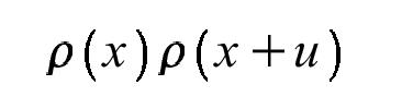
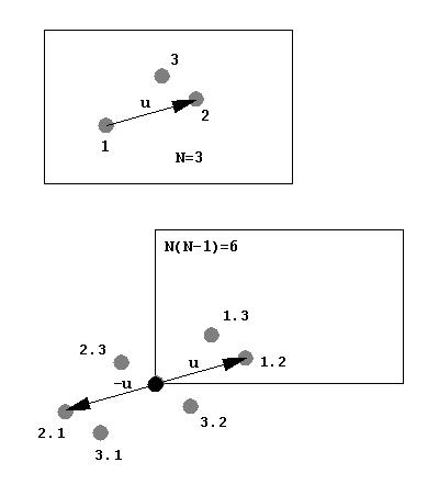
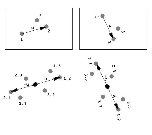
will only be non-zero where the position vector (x) lies at an atom and (x+u) also lies at an atom. Specifically, u will be an interatomic vector (or intra-atomic if it has length zero). Note that since we integrate over x, the locations of the atoms are not important, but their relative positions are (the tails of all the u vectors are at the origin):
We use precisely this interpretation of the Patterson function in MIR and MAD techniques to find heavy atom sites. Thus the Patterson inherently contains information about the structure, since it contains the sum of all interatomic vectors. An important thing to note is that Patterson is a function of vector length/direction (u) but not the location of the atoms (x). This is important for the Rotation Function, which relies on independence of position of the molecule but the precise relative position of the atoms within it. The weighting is just the product of the electron densities at the atoms.
Some properties of the Patterson:
The Patterson is dense because the number of peaks is N2. Therefore, hand interpretation of the Patterson for large biological molecules is impossible (Dorothy Hodgkin solved vitamin B12 that way): triclinic hen-egg lysozyme has 1001 atoms (excl waters) and 1,001,000 non-origin Patterson peaks. However the vector information is still there, and the Rotation Function (RFn) makes use of it.
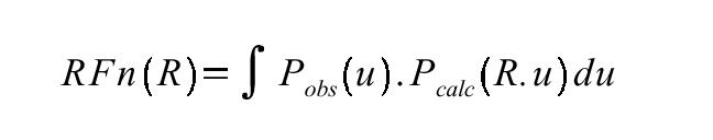
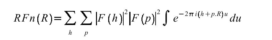
The RFn (Rossmann, M. G., D. M. Blow. 1962. The detection of sub-units within the crystallographic asymmetric unit. Acta Crystallogr. 15:24-31) is a simple product function that compares an observed and model Patterson function for a given trial rotation. The calculation is integrated over a certain volume U in Patterson space. The second form of the equation is the equivalent in reciprocal space. The RFn is conventionally evaluated over a 3-D grid of angles (e.g. α, β, γ). Pattersons conceptually contain two types of interatomic vectors: intramolecular and intermolecular. The RFn works because intramolecular vectors are dependent only on molecular rotation, not molecular translation. Therefore at least some component of the Patterson is independent of translation. RFns take advantage of the fact that intramolecular vectors will be on average shorter than intermolecular vectors, so excluding longer vectors from the search improves the signal to noise. The usual volume is a sphere around the Patterson origin: typical values are 40-70% of the molecular diameter (e.g. 16-27 Ångstroms). The principal parameters you vary in RFns are the resolution range and this radial cutoff. There's also often an inner radial cutoff to remove artefacts from the very large origin peak of the Patterson.
Although I talk about intra and interatomic vectors, they aren't separable in the Patterson, just conceptual contributions to the function itself.
The conventional RFn is still a slow calculation, but Tony Crowther (Crowther, 1972) showed how the calculation may be approximated by spherical harmonics and proceed via a single Fast Fourier Transform (FFT) step. This so-called Fast Rotation Function has been further refined by Jorge Navaza (Navaza, 1994, Acta Cryst. A50, 157-163). The programs MERLOT, ALMN, POLARRFN, MOLREP and AMORE use the Fast Rotation Function. CNS and X-PLOR use the conventional RFn. Every Fast Rotation Function I know of is parameterised in terms of (α,β,γ). The programs BEAST (Read, 2001, "Pushing the boundaries of molecular replacement with maximum likelihood." Acta Cryst. D57: 1373-1382.) and PHASER (J. Appl. Cryst. (2007). 40, 658-674. Phaser crystallographic software. A. J. McCoy, R. W. Grosse-Kunstleve, P. D. Adams, M. D. Winn, L.C. Storoni & R.J. Read) use a different maximum likelihood function for it's RFn which is scored in terms of Log Likelihood Gain (LLG) and resists direct comparison with other methods. The details of the algorithms may vary, but the central idea is the same.
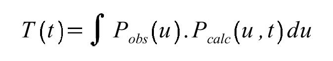
You don't have to use this sort of rotation function. In principle, you can calculate the correlation between the model Fcalc and the Fobs with the model in a P1 cell of the correct cell dimensions. Ideally this should show a peak where the model matches one orientation of a molecule in one asymmetric unit of the unit cell. Being in P1 it's also independent of translation, at least for the first molecule. Unfortunately there's no very quick way to do this and such a search is inherently very slow. It is more usual to use the R-factor and correlation coefficients for this method to score and rank the output of more conventional rotation functions. (The correlation coefficient over a narrow resolution range is closely related to a correlation between two origin-removed Pattersons and so is sometimes referred to as the Patterson Correlation - especially in the context of CNS/X-PLOR).
Despite using self-rotation functions in the first protein structure I solved, I personally don't find self-rotation functions all that much use for regular proteins. (Because you still have to have a good model to solve the cross-rotation function). But for viruses they are often used to establish the orientation of the viral capsid within the unit cell, and can provide enough information to start ab initio phasing. In lower-symmetry cases, they can tell you the direction of the non-crystallographic symmetry (NCS) but the self-rotation function cannot tell you the location of the axis.
If you can get decent NCS information from the self-rotation function or other methods (e.g. heavy atom sites), the program GLRF (Tong and Rossman, 1990) can use this information to try and screen for NCS-related cross-rotation function peaks. It's also a fairly straightforward (albeit non-trivial and nit-picking) case to write your own program to screen sets of peaks.
One of the more informative plots out of the self-rotation function is the stereographic projection. This plots the values of the function at a given κ (axis rotation angle) for φ and ψ. However the plot is constructed to that it appears as if it were projected onto a hemisphere and viewed from above (from +z toward the origin). These sections have ψ = 0 or 180 at the centre, ψ = 90 around the edge, and φ as marked around the periphery. Example using POLARRFN:
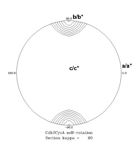
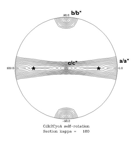
These sections are contoured from 0.4 of the origin peak by 0.05. In the 2-fold (κ=180) section, the crystallographic axes are: c/c* along z (middle of the plot); a/a* along x (ψ=90, φ=0), right edge of circle; b/b* along y (ψ=90, φ=90), top edge of circle. On the 2-fold section the crystallographic axes for P212121 are evident, plus there's a ridge of density in the b/c plane. The 4-fold (κ=90) section gives us a clue why this is - there's a pseudo-4-fold NCS axis along b, which means the crystal locally impersonates point group 422 and there must be an additional 2-fold NCS-axis at (ψ=45, φ=90, κ=180) and (ψ=45, φ=270, κ=180) (marked with * on the plot). [Note: a 2-fold axis at 45 degrees from another 2-fold generates a 4-fold in the direction of their cross-products]
In this example, and quite typically, the precise location of the NCS axis is somewhat obscured by smearing, and finding NCS axis close to crystallographic axis is usually somewhat of a challenge.
PC refinement is designed to improve the solution in the case where the model has internal degrees of flexibility that can be modeled as rigid-body movements. An early application of this was Fab domains, which usually behave as rigid Fv (VH+VL domains) and Constant domain (CH1+CL) rigid bodies connected by a restricted axis of movement - the "hinge". See, for example: Ban et al. (1994) "Crystal Structure of an Idiotype-Anti-Idiotype Fab Complex" PNAS 91, pp. 1604-1608. PC refinement has sometimes produced spectacular gains, but it's usage seems to have diminished somewhat in recent years. It doesn't help that CNS and X-PLOR have very slow molecular replacement implementations compared to programs like AMORE and PHASER. An alternative to PC refinement would be breaking the model up into Fv and Constant domains, but this potentially has a reduced signal/noise power than a larger model that is fairly close to the correct orientation.
which basically measures the similarity between the observed and calculated Pattersons, measured over the entire Patterson asymmetric unit. The T2 variant of this function subtracts off the "known" intramolecular vector component calculated from the model. The T and T2 functions can be quickly calculated in a single FFT pass and remain the searches of choice for really fast screening for MR solutions. Many variants of the original functions have been proposed including the TO/O function (Harada et al., 1981) that contains some factors against molecular interpenetration.
A conceptually simpler method is to compare the R-factor and correlation coefficient of Fobs and Fcalc at every point on the grid search.
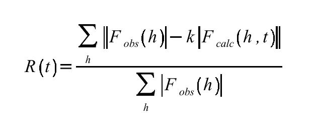
These calculations are slow since they involve comparison of reflection lists at each TFn grid point, and programs like AMORE (Navaza, 1994) tend to use the R-factor and correlation only as screening parameters in peaks found in T and T2 searches. However if speed is not an issue, correlation coefficient searches are often extremely effective. Correlation coefficients are usually more useful than R-factors because they appear to be more sensitive to MR solution quality in the range of model errors typically encountered during molecular replacement. Except in very favorable cases (where pretty much anything would work) the MR solutions can have near-random R-factors at this stage and the difference between correct and incorrect is often very small in R-factor space. This distinction in correlation coefficient is often more pronounced.
Where you have experimental phases (e.g. poor MIR or MAD phases that aren't quite enough to interpret the map) then a phased translation function can be utilised that compares not only amplitudes but also phases between the observed and calculated data.
One last form of translation function is the packing function (Hendrickson and Ward, 1976). This is a simple steric function that allows one to delimit viable regions for potential translation function solutions. The Uppsala program PACMAN allows trivial screening of AMORE solutions based on packing criteria, for example. However generally speaking packing functions are not very sensitive and are used only as secondary criteria - it's not uncommon for models to differ from real structures in surface loops, which is precisely where the first packing "clashes" occur in such tests. Used intelligently it is however possible to use packing functions to screen potential solutions.
The program EPMR (Kissinger et al., 1999, "Rapid automated molecular replacement by evolutionary search", Acta Crystallographica, D55, 484-491) inherently does 6-D searches using a Genetic Algorithm. Genetic Algorithms work by generating a "population" of possible solutions represented as strings of bits encoding the solution. The Genetic Algorithm (GA) then manipulates these solutions using operators on the bit strings that mimic genetic processes like mutation, recombination etc. Although this sounds an unlikely algorithm, GAs can optimise functions very effectively (I wrote a GA version of the TFn program BRUTE that often found solutions in 1/100th of the time of the conventional program). The scoring function in EPMR is a combination of correlation coefficient and packing function. Some people have been enthusiastic about EPMR but in my hands it's not proven to be any better than more conventional methods. GA is also inherently partially driven by random numbers and it would be fairly easy to skip right past the real solution simply by not sampling that part of 6D space.
| PHASER | Rotation and translation functions using hybrid maximum likelihood scoring method with tradition "fast" RFn and TFn methods. Fairly fast and I now use this program almost exclusively for molecular replacement efforts. Included in Phenix, CCP4 suites. |
|---|---|
| MOLREP | Rotation and translation functions with many of the features of AMORE, extra special features for multiple molecules in the asymmetric unit. Part of CCP4 suite. |
| EPMR | Genetic algorithm 6D search. Some people swear by it. I've never had it solve anything that AMORE or PHASER couldn't handle. Slow. The new OpenEPMR has open availablility. |
| AMORE | Rotation and translation functions, including facilities for searching long lists of possible solutions. Very fast. Recommended. Can search for more than model of more than one type to assemble multidomain solutions. Currently part of CCP4. |
| CNS | Uses Patterson-based RFn and TFn implementations which tend to run slowly. It's main advantage is PC refinement which allows optimisation of internal degrees of freedom in a model prior to the translation function. |
| BEAST | Rotation and translation functions using a new maximum likelihood scoring method. I've not much experience with this program so it's applicability is difficult to assess. This was essentially the precursor to PHASER. |
| GLRF | Global Locked Rotation Function that allows inclusion of non-crystallographic symmetry constraints in MR searches. The programs REPLACE and COMO seem to be offspring of this program. See Tong and Rossman (1990). |
| Mr BUMP | An unlikely name for an automated Molecular Replacement pipeline program using MOLREP or PHASER. http://www.ccp4.ac.uk/MrBUMP/. |
| BALBES | Molecular replacement pipeline suite. http://www.ysbl.york.ac.uk/~fei/balbes/ |
| MERLOT | The first MR program suite. Now completely supplanted by PHASER, AMORE, MOLREP etc. |
| ALMN | Fast RFn program using the Crowther algorithm for cross-rotation searches. Results expressed as Eulerian angles. Part of CCP4 suite. |
| POLARRFN | Fast RFn program using the Crowther algorithm for self- and cross-rotation searches. Results expressed as Polar angles. Most useful for self-rotation searches where the angle system makes the symmetry easier to interpret. Part of CCP4 suite. |
Previously, I recommended AMORE since it is fast and I had extensive experience with it. Currently I wholeheartedly recommend PHASER which I have used for all of my recent molecular replacement structure determinations. I only ever consider slower programs if the problem is very difficult, at which point probably none if them will work anyway. MOLREP is probably every bit as powerful as AMORE, but the command file syntax is extremely arcane (at least to my eyes). It may be even as good as PHASER but PHASER syntax is much more human readable.
that comes out to about 29% identity. This is somewhat of a conservative estimate, but models with only 10% identity are going to give you a really hard time. The fastest check for similar sequences with the PDB database is to use a BLAST/FASTA server with a PDB sequence database. The alignments can also give you ideas on divergent loops which you can omit from the model. You can then align these potential models onto each other (perhaps with DALI or LSQMAN) and see which bits are more similar and which are more divergent.
Homology models do not, in general, work. You are welcome to try them, but if you're desperate enough to want to try, your starting model isn't very good and the homology model is unlikely to make it any better. Homology modeling programs include MODELER and the PHYRE server (see below). The program ROSETTA has been known to generate models accurate enough for molecular replacement, but ROSETTA takes a long time to run and it's not exactly a trivial process to install and configure it (Rigden DJ, Keegan RM, Winn MD (2008) Acta Cryst. D64, p.1288-91).
NMR models are often problematic. Using either average NMR structures or an ensemble NMR structure (in something like PHASER that supports this method) is often a frustrating exercise, despite the fact that you'd think that complementary techniques should generate similar structures. The obvious snark is that NMR generates structures with higher error levels than are immediatley apparent, but whatever the reason things are often more difficult with NMR models. See: Chen YW, Dodson EJ, Kleywegt GJ (2000) Structure, Vol. 8, p.213-20.
There are a number of things that will improve your chances of success:
Differing sequences: where sequences differ, some people leave the old side-chains on, some replace them with the new sequence, and some chop them to Alanine or Serine. To me, the Ala option is always the last one, because even if the Leu in the model is really an Asn in the unknown, Leu doesn't look that much different to Asn at 3.5 Ångstrom resolution. But it does look rather different from Ala. Often the side-chain orientations will overlap at least partially. Replacing side-chains with the right sequence makes sense only when you have a pretty good idea of where the side-chain will go, otherwise you are more likely to increase the error in your model. Some people have also found use in Cα-only models, although I fail to see why this would be better than poly-Ala and I think in most cases it would be considerably worse. The CCP4 program CHAINSAW will use a sequence alignment to edit your model for you, but you should use this in addition to - not instead of - your own guesses about the structure.
Multiple sequence alignments may help to you discriminate between more and less-highly conserved parts of the structure. Careful inspection of the model may reveal areas with high B-factors or crystal packing interactions which may benefit from being removed. In rare cases where you can get a partial molecular replacement solution, refined B-factors of the partial solution can also be a guide. (I did this with one structure here at Princeton, which was necessary to attain a solution). Multipe sequence alignments may benefit from using sophisticated algorithms like PFAM to find the correct alignment in low-homology cases: the standard BLAST method has its limitations. Be aware that sequence searches are driven in sequence space and so may not make the most natural domain boundaries within structures - PFAM in particular tends to be a little tighter than the limits on most domains.
For surface loops, especially ones that have insertions and deletions, it may make sense to remove them. However don't get carried away: things with different sequence often have similar structure, and the smaller the model gets the worse are your chances of finding the right solution. Without knowing the correct solution it's difficult to assess whether you are improving your model or making it worse, so it always pays to check a wide range of model edits.
If you have a lot of similar models, you can even try the "ensemble" approach where you superimpose a whole set of slightly divergent structures to produce an "averaged" model. Wayne Hendrickson did this when solving CD8 with antbody Fv fragments (Leahy et al., 1992), lacking any other molecules of close homology. In the case of NMR structures you can use the ensemble, the average minimised structure or each of the models in turn - or indeed any and all of these approaches. PHASER allows the fairly trivial accumulation of pre-aligned PDB files to construct an ensemble for MR searches. The most radically successful example of this in my personal experience was finding the WD40 domain 'B' subunit of the PP2A ABC holoenzyme despite minimal sequence homology with the actual structures I used. The placement was confirmed with low resolution phases from a Ta6Br12 derivative.
If you have models with known internal degrees of freedom, it can be an advantage to place the axis of the internal rotation along the Z axis. This technique was taught to me by Steven Sheriff who used it to simplify his antibody Fab molecular replacement solutions by putting the elbow axis approximately parallel to Z. Split peaks arising from conformational change about that internal rotation will show differences only in γ within the α,β,γ Eulerian angle formalism. Be aware that AMORE will, by default, re-orient your model for you. Use TABFUN NOROTATE to prevent that. I've used this method, back in ye olde days when I used to solve Fab structures, to find solutions that were clearly "paired" between Fv and constant (Cl:Ch1) domain models. PHASER doesn't re-rotate your models so this should be easier.
Also, for multi-domain models, often it works better to split models up into individual domains, particularly where the sequence identity is relatively high. If the degree of internal flexibility is not great, it may also pay to use AMORE's TABFUN NOROTATE to keep the models in the same relative orientation so you can potentially find related peaks in the rotation functions for the separate models. Note that the signal/noise of RFn and TFn peaks inevitably goes down as you reduce the size of the model, so don't do this in the absence of some evidence for conformational flexibility.
The CCP4 program CHAINSAW (N. Stein, J. Appl. Cryst. 41, 641 - 643 (2008).) will attempt to automatically edit your model for you. If you're feeling braver the PHYRE server at http://www.sbg.bio.ic.ac.uk/~phyre/ will generate a homology model for you as a starting point. (Kelley LA and Sternberg MJE. Nature Protocols 4, 363 - 371 (2009)).
It's in a crystal, so it has to pack well. This is actually a very sensitive criterion although one that is equally beholden to the incorporation of incorrect features (e.g. long loops) in your search model. Programs like PHASER actually use packing criteria to exclude badly-packing solutions, but this is not quite the same as excluding solutions with obviously farcical packing. Simply display the solution in O or COOT in the context of the unit cell symmetry and see if it packs. Minor clashes from surface loops might be OK since these are likely to diverge between structures. Larger-scale clashes are probably indications of errors. If the molecule is swimming on it's own in the middle of the asymmetric unit without touching anything, you've probably underestimated the number of molecules in the asymmetric unit. Gerard Kelywegt wrote an auto-amore script featuring an automatic filtering of packing via the program PACMAN, but this program doesn't always seem to be bug-free. The program PHASER does a packing check my default, which is very useful to separate out the clearly wrong from potentially correct solutions but some correct models can generate significant packing errors if there is one loop that is different in a region of close contact. The PHASER "PACK" command can increase the number of acceptable clashes before a potential solution is rejected.
I used to say that "if the correlation coefficient is > 0.4, you've solved it" but there are too many exceptions to that, including blatantly wrong solutions that fail the packing test, above. In PHASER the advice tends to be case in terms of the signal/noise (Z score) of the solution (see: Has Phaser Solved It?). What you're really looking for is discrimination - i.e. a peak so strong that it is obvious that it is the right one because there are no others near it in the RFn or TFn map. For solutions of the same molecule (identical sequence) in different crystal forms that should be accompanied with a correlation coefficient of >0.6 and an R-factor in the 35-45% range. With PHASER this would mean an LLG>100 and a Z-score > 10. For more divergent models anything with a correlation coefficient >0.35 is worth considering. I'm not sure that I've ever personally found a good MR solution of the entire asymmetric unit with a correlation coefficient of worse than 0.35 (partial contents and bad models are a different story). For PHASER, the LLG and in particular the Z-score (>5) are good guides, but again, the number of peaks in the RFn and TFn is probably one of the most revealing criteria (and probably related to the Z-score). In PHASER the LLG is sensitive to the expected RMS between the model and unknown structure and so really isn't an independent measure of success.
Ultimately, however, the One True Test of the usefulness of any solution is if the phases show you something in the electron density map that wasn't in your model. Refining 100 potential solutions to see if that is the case can be a little tedious, but if all else fails one can try that.
Scaling of diffraction data only tells you what your point group is (and if it is a P,C,F,I,R lattice). Usually there is more than one possible space group to try, and to be thorough you should try them all. However if you are short of time or very confident in your data you can sometimes reduce the number of potential space groups by utlising information about systematic absences. Pure rotation axis do not cause any systematic absences. Screw axis do cause them:
| Screw | Absences |
|---|---|
| 21 | (0,0,l) != 2n |
| 31 | (0,0,l) != 3n |
| 32 | (0,0,l) != 3n |
| 41 | (0,0,l) != 4n |
| 42 | (0,0,l) != 2n |
| 43 | (0,0,l) != 4n |
| 61 | (0,0,l) != 6n |
| 62 | (0,0,l) != 3n |
| 63 | (0,0,l) != 2n |
| 64 | (0,0,l) != 3n |
| 65 | (0,0,l) != 6n |
This table assumes the symmetries are along c* (i.e. the l index) but some space groups may show them on other axes e.g. in P21 the absences are on (0,k,0) because the 21 axis is along b/b*. Be aware however that I have been fooled by systematic absences more than once even during my time here at Princeton, and by far the best way is to check all the possible space groups - after all, if the right space group doesn't become obvious amongst a list of possible space groups, it's probably not a good MR solution.
You may need to permute your a/b/c axes to check all space groups. For example, arbitrary data in a primitive orthorhombic space group (i.e. point group 222) you need to test:
Note that you can't tell the difference between enantiomorphs (e.g. P3121 and P3221 are enantiomorphs) without actually solving the structure (or heavy atom substructure). They have both the same systematic absences and all other intensity statistics (except the R-factors and correlation coefficients during molecular replacement).
PHASER makes a number of choices for you: the size of the rotation grid and the integration radius being two of them, which it extracts from the extent of coordinates in the given PDB files. PHASER uses a Log Likelihood Gain (LLG) as the scoring function which represents the extent to which the model gives a better prediction of the actual data than a random array of atoms. PHASER reports the raw LLG but also the "Z score" which is essentially the signal to noise of the peak(s) in the rotation and translation functions. LLG is modulated by your estimate for the similarity of the structures, either given as expected RMS or % sequence identity.
There are three models: the structure of the A subunit of PP2A previously solved by David Barford's group but broken into two pieces based on fortuitous guesswork (Groves et al (1999) Cell 96: 99-110; PDB code 1B3U); the structure of PP-1 catalytic subunit (Goldberg et al (1995) Nature 376: 745-753; PDB code 1FJM). I did manage to solve it with the intact PP2A-A subunit but it was clear that the C-terminus was misplaced. As it happens my arbitrary cut at 460/461 was pretty close to ideal.
The straightforward script file defines the source of the data (HKLIN, LABIN), the resolution, the size of the asymmetric unit (COMPOSITION), the sources of the three different models and their sequence identity with the target (ENSEMBLE) and in this first pass we ask PHASER to find the N-terminal part of PP2A-A (1b3u_AN.pdb). The identity is really 100% but we want to downgrade that estimate to allow a little structural variation:
phaser << EOF
MODE MR_AUTO
HKLIN ac101_truncate.mtz
LABIN  F=F SIGF=SIGF
RESOLUTION 20.0 4.0
COMPOSITION PROTEIN MW 90000 NUMBER 2
SGALTERNATIVE ALL
ENSEMBLE ensemb1 PDBFILE 1fjm_A.pdb IDENT 47.0
ENSEMBLE ensemb2 PDBFILE 1b3u_AN.pdb IDENT 90.0
ENSEMBLE ensemb3 PDBFILE 1b3u_AC.pdb IDENT 90.0
SEARCH ENSEMBLE ensemb2 NUMBER 1
ROOT example1
PACK 10
EOF
SGALTERNATIVE ALL tells the program to consider alternatives. In this case this is only I222 and I212121. What follows are heavily edited highlights of the output. During the rotation function:
------------------------------
FAST ROTATION FUNCTION #1 OF 1
------------------------------
(snip)
   Performing a 3.48936 degree search.
   0%                                                    100%
   |=====================================================| DONE

   Top 32 rotations before clustering will be rescored
   0%                                100%
   |=================================| DONE
the program finds a total of 32 peaks above the default criteria of 75% of the top peak. This is a very low peak count which suggests already that it's found the molecule. This is confirmed by a summary of the results:
   There was 1 site over 75% of top
   The sites over 75% are:
   #     (#)   Euler1 Euler2 Euler3   LLG   Z-score Split #Group   raw/top
   1     1       88.0   86.5  266.5 +100.76    5.61   0.0     25 100.0/100.0
                268.0   86.5  266.5
                272.0   93.5   86.5
                 92.0   93.5   86.5
where it finds one unique peak (the different Eulerian angles are symmetry-related) at a good +ve LLG and an OK Z-score (>5 is
good but not epic). Now we must run the Translation Function in each of the two possible space groups, which PHASER does for
us:
   Space-Group Name (Number):   I 2 2 2 (23)

---------------------------------
FAST TRANSLATION FUNCTION #1 OF 1
---------------------------------

   There was 1 site over 75% of top
   The sites over 75% are:
   #     (#)   Frac X Frac Y Frac Z   LLG   Z-score Split #Group    raw/top
   1     1      0.640  0.921  0.196 +180.60   12.31     0      1 305.29/305.29
which are edited highlights of the output and you'll notice that in I222 there's a single TFn peak, a bigger LLG, and a pretty good Z-score (12 suggests a high confidence in the solution). But of course we must compare this with I212121:
   There were 18 sites over 75% of top
   The sites over 75% are:
   #     (#)   Frac X Frac Y Frac Z   LLG   Z-score Split #Group    raw/top
   1     1      0.389  0.288  0.196  +98.94    7.89     0      1 225.53/225.53
   2     2      0.388  0.220  0.196  +87.72    7.19    13      1 220.95/220.95
   3     3      0.389  0.083  0.196  +84.89    7.02    32      1 215.70/215.70
   4     7      0.390  0.015  0.196  +84.36    6.98    44      1 205.58/205.58
   5     4      0.389  0.108  0.196  +81.67    6.82    29      1 213.48/213.48
   6     12     0.389  0.002  0.197  +81.17    6.79    46      1 202.44/202.44
   7     5      0.389  0.904  0.196  +77.81    6.58    37      1 209.36/209.36
   8     6      0.389  0.308  0.196  +76.56    6.50     4      1 207.70/207.70
   9     14     0.535  0.922  0.446  +76.24    6.48    39      1 198.59/198.59
   10    9      0.388  0.826  0.196  +75.92    6.46    31      1 204.57/204.57
   11    8      0.389  0.257  0.197  +74.29    6.36     6      1 205.21/205.21
   12    10     0.389  0.244  0.196  +74.28    6.35     9      1 203.69/203.69
   13    20     0.390  0.195  0.196  +72.56    6.25    18      1 194.57/194.57
   14    15     0.389  0.938  0.196  +72.40    6.24    42      1 197.50/197.50
   15    11     0.388  0.982  0.196  +71.78    6.20    48      1 202.57/202.57
   16    13     0.388  0.129  0.197  +71.44    6.18    26      1 198.59/198.59
   17    19     0.389  0.053  0.197  +70.12    6.10    37      1 195.78/195.78
   18    18     0.388  0.893  0.196  +68.51    5.99    36      1 196.00/196.00
which has more peaks, lower LLGs and lower Z-scores. I222 is clearly the "winner" here. PHASER then goes on and refines the solution against all the data in the MTZ file:
   Refinement Table: Space Group I 2 2 2
   -------------------------------------
   #+ = input number    #* = output number
   Unsorted (refinement order)       Sorted in LL-gain order
       Initial   Refined                     Initial   Refined
   #+  LL-gain   LL-gain   Unique    #*  #+  LL-gain   LL-gain   Unique  =#*
   1   307.42    320.16    YES       1   1   307.42    320.16    YES
and outputs a ".sol" file reflecting the partial solution:
#  [No title given]
SPACegroup HALL  I 2 2 #I 2 2 2
SOLU SET  RFZ=5.6 TFZ=12.3 PAK=0 LLG=224 LLG=320
SOLU 6DIM ENSE ensemb2 EULER   88.937   87.095  267.296 FRAC -0.35006 -0.08334  0.20192
Now we must find the locations of the other two models, in reference to this one. The script is essentially the same except that we ask it to find a different model (ensemb3) in the presence of the existing solution (example1.sol, ensemb2 as before) and we no longer need it to check all possible space groups:
phaser << EOF
MODE MR_AUTO
HKLIN ac101_truncate.mtz
LABIN  F=F SIGF=SIGF
RESOLUTION 20.0 4.0
COMPOSITION PROTEIN MW 90000 NUMBER 2
ENSEMBLE ensemb1 PDBFILE 1fjm_A.pdb IDENT 47.0
ENSEMBLE ensemb2 PDBFILE 1b3u_AN.pdb IDENT 90.0
ENSEMBLE ensemb3 PDBFILE 1b3u_AC.pdb IDENT 90.0
SEARCH ENSEMBLE ensemb3 NUMBER 1
ROOT example2
@example1.sol
PACK 10
EOF
You can do this via the GUI in CCP4 (and perhaps even in Phenix) but it's easy to do via command line...... Once more, edited output highlights:
------------------------------
FAST ROTATION FUNCTION #1 OF 1
------------------------------

Top 200 rotations before clustering will be rescored

   There were 10 sites over 75% of top
   The sites over 75% are:
   #     (#)   Euler1 Euler2 Euler3   LLG   Z-score Split #Group   raw/top
   1     51      21.3   11.8  318.9 +239.66    3.19   0.0      9  79.0/ 79.0
                201.3   11.8  318.9
                338.7  168.2  138.9
                158.7  168.2  138.9

(etc)

---------------------------------
FAST TRANSLATION FUNCTION #1 OF 1
---------------------------------

   Fast Translation Function Table: Space Group I 2 2 2
   ----------------------------------------------------
   #SET #TRIAL      Top    (Z)    Second    (Z)     Third    (Z)    Ensemble
      1      1   216.17 ( 5.53)   207.64 ( 4.96)   204.61 ( 4.75)   ensemb3
      1      2   386.85 (16.92)        -      -         -      -    ensemb3
      1      3   211.40 ( 5.63)   209.95 ( 5.53)   209.01 ( 5.47)   ensemb3
      1      4   212.17 ( 5.58)   211.56 ( 5.54)   209.75 ( 5.42)   ensemb3
      1      5   217.19 ( 5.83)   207.89 ( 5.18)   207.88 ( 5.18)   ensemb3
      1      6   207.41 ( 5.34)   203.82 ( 5.08)   203.71 ( 5.07)   ensemb3
      1      7   208.58 ( 5.39)   208.40 ( 5.37)   206.48 ( 5.24)   ensemb3
      1      8   208.94 ( 5.32)   208.09 ( 5.27)   206.49 ( 5.16)   ensemb3
      1      9   213.57 ( 5.76)   209.15 ( 5.45)   208.65 ( 5.42)   ensemb3
      1     10   208.04 ( 5.17)   207.52 ( 5.13)   204.76 ( 4.95)   ensemb3
   ---- ------
So this rotation function doesn't fare as well - 200 peaks with 10 after clustering, not a very hight Z-score although the
LLG is reasonable because this is done in the presence of the existing PP2A-A:N solution. PHASER doesn't need any prompting to
take each of the 10 RFn solutions and use them in the TFn. In fact you can see that the second peak in the RFn is clearly the
best one with the Z-score and LLG both indicating clearly which is the correct solution. This then quickly becomes the
rigid-body refined solution in "example2.sol":
#  [No title given]
SPACegroup HALL  I 2 2 #I 2 2 2
SOLU SET   RFZ=5.6 TFZ=12.3 PAK=0 LLG=224 LLG=320 RFZ=2.9 TFZ=16.9 PAK=1 LLG=424 LLG=707
SOLU 6DIM ENSE ensemb2 EULER   88.860   87.146  267.299 FRAC -0.35038 -0.08292  0.20225
SOLU 6DIM ENSE ensemb3 EULER   98.877  115.689  270.499 FRAC -0.23492  0.06151  0.30440
which has a refined LLG of 707 against all the data. And now onto the final model, finding the PP2A:C subunit with the PP1 model. Unlike looking for PP2A:A with PP2A:A the homology here is not 100% but the identity is high enough that we expect pretty reasonable similarity in structure:
phaser << EOF
MODE MR_AUTO
HKLIN ac101_truncate.mtz
LABIN  F=F SIGF=SIGF
RESOLUTION 20.0 4.0
COMPOSITION PROTEIN MW 90000 NUMBER 2
ENSEMBLE ensemb1 PDBFILE 1fjm_A.pdb IDENT 47.0
ENSEMBLE ensemb2 PDBFILE 1b3u_AN.pdb IDENT 90.0
ENSEMBLE ensemb3 PDBFILE 1b3u_AC.pdb IDENT 90.0
SEARCH ENSEMBLE ensemb1 NUMBER 1
ROOT example3
@example2.sol
PACK 10
EOF
And this should work pretty much as the same as finding the second molecule.... except that you hope with the whole of PP2A:A in place now the discrimination should be even easier:
------------------------------
FAST ROTATION FUNCTION #1 OF 1
------------------------------

   Top 16 rotations before clustering will be rescored

   There were 2 sites over 75% of top
   The sites over 75% are:
   #     (#)   Euler1 Euler2 Euler3   LLG   Z-score Split #Group   raw/top
   1     1      105.8   63.2    5.2 +463.45    6.15   0.0     11 100.0/100.0
                285.8   63.2    5.2
                254.2  116.8  185.2
                 74.2  116.8  185.2
   2     2      101.4   62.4   11.4 +460.43    5.82   5.8      1  91.0/ 91.0
                281.4   62.4   11.4
                258.6  117.6  191.4
                 78.6  117.6  191.4

---------------------------------
FAST TRANSLATION FUNCTION #1 OF 1
---------------------------------

   Fast Translation Function Table: Space Group I 2 2 2
   ----------------------------------------------------
   #SET #TRIAL      Top    (Z)    Second    (Z)     Third    (Z)    Ensemble
      1      1   967.06 (32.25)        -      -         -      -    ensemb1
      1      2   922.55 (31.14)        -      -         -      -    ensemb1
   ---- ------

----------------
PRUNE DUPLICATES
----------------

   Refinement Table: Space Group I 2 2 2
   -------------------------------------
   #+ = input number    #* = output number
   Unsorted (refinement order)       Sorted in LL-gain order
       Initial   Refined                     Initial   Refined
   #+  LL-gain   LL-gain   Unique    #*  #+  LL-gain   LL-gain   Unique  =#*
   1   967.06    1060.63   NO        1   2   922.55    1060.65   YES
   2   922.55    1060.65   YES           1   967.06    1060.63   NO      1
Starts out with relatively few RFn peaks, which is promising. It finds a very good TFn solution for both peaks - however
we are expecting only the one peak. It refines each potential solution (each of them a set of 3 structures from different
PDB files) and in the final round of refinement determines that the two solutions are equivalent to each other (related
by symmetry) and so finds a unique solution. You can see the relationshop if you look at the peaks - basically the two
RFn solutions are from a single split peak. And so there you have it - it take 3 command files, each one derived from the
other, to generate a fairly straightforward molecular replacement solution requiring relatively little manual intervention
as far as parameters are concerned.
In testimony to just how straightforward working with PHASER is, I solved this structure at the beamline just after collecting and processing the data. PHASER requires a lot fewer steps than AMORE, and usually doesn't require a lot more manual intervention than the small script I showed above. In favorable cases it is generally quite fast, but for larger structure with weaker models it can take a while - the 20S proteasome structure which required finding a lot of subunits/rings in a very large unit cell took quite a few hours of CPU to work through all the various permutations. For each of the scripts PHASER writes out an MTZ file and PDB file for the partial solution. You can look at maps or check the appearance of the model. PHASER triest to cluster the solution around each other - this doesn't necessarily mean it connects the fragments correctly, but if you load it into COOT and "write symmetry coordinates" it doesn't take long to assemble a covalently contiguous solution in those cases were PHASER hasn't already come up with one.
This was a pseudo hetero-trimeric case. In the case of homomultimers you can request that PHASER find all N copies, which it does sequentialy in a manner similar to what I did above. The downside is that if it fails you don't get a PDB file of the intermediate solution (at least, not by default) so I usually prefer to look for one monomer at a time unless I'm very confident of the outcome.
Let's assume we have the native data in MTZ (CCP4) format via SCALEPACK2MTZ or a similar step. AMORE requires a reformatting step to get the data into AMORE-usable format:
amore HKLIN tetHEL_1.mtz HKLPCK0 tethel.hkl <<  eof >! prep.amore
SORTFUN RESOL 20.  2.8
LABI FP=FP  SIGFP=SIGFP
eof
We include the resolution to a little greater than we anticipate using during the searches.
Now we chose a model. We simply hack out the first molecule from the PDB file (pdb1jj3.ent) and call it model.pdb (residues A1-A129, 1001 atoms). AMORE by default centers (at origin) and re-orients the model, as well as calculating some reflection data. Note that here we must enter the unit cell for the target molecule.
amore  XYZIN1  model.pdb \
       XYZOUT1 searchrot.pdb \
       TABLE1  search.tab << eof >>! prep.amore
VERBOSE
TABFUN
CRYSTAL 79.22  79.22  38.06 90 90 90 ORTH 1
MODEL 1 BREPLACE 0 BADD 0
SAMPLE 1 RESO 2.8 SHANN 2.5 SCALE 4.0
eof
Now we can run rotation functions. Calculation of the Matthew's
coefficient or running the CCP4 program WILSON allows us to deduce that
we are looking for only one molecule in the asymmetric unit. Therefore
there is no point running a self-rotation function. We run a cross
rotation function:
amore  TABLE1  search.tab \
       HKLPCK1 search.hkl \
       hklpck0 tethel.hkl \
       CLMN1   search.clmn \
       CLMN0   tethel.clmn  \
       MAPOUT  amore_cross.map <<  eof >! rfn.amore
ROTFUN
VERBOSE
TITLE : Generate HKLPCK1 from MODEL FRAGMENT   1
GENERATE 1   RESO 10.0 3.0  CELL_MODEL 75. 75. 75.
CLMN CRYSTAL ORTH  1 FLIM 0.E0 1.E8  SHARP 0.0 RESO  10.0 3.0 SPHERE 18
CLMN MODEL 1         FLIM 0.E0 1.E8            RESO  10.0 3.0 SPHERE 18
ROTA  CROSS  MODEL 1  BESLIMI 6 120 STEP 2.5 PKLIM 0.5  NPIC 100 BMAX 90
eof
Note that we select a small radius cutoff (18 Angstrom) and use data to
3.0 Angstrom. Normally I use no better than 3.5 Angstrom for molecular
replacement unless the model is very good, as in this case. Often the
native data doesn't go that far, either. It's often advantageous,
as here, to drop the lowest resolution reflections since they are
dominated by solvent effects and are sometimes not well measured
close to the beamstop. The CELL_MODEL is set to a cubic (i.e. a=b=c)
cell of 75 Angstroms on an edge. The model structure factors are
calculated in this cell. It must be at least the maximum diameter
of the molecule plus the radius cutoff value, to ensure that there
are no intermolecular vectors from the model within the radius cutoff
you specified. In this case the model is maximum ~52 Angstrom wide
so 70 is the minimum and we pad it a little. The program PHASER
decides this for you, but in AMORE you must decide it for yourself.
A quick and simple way to inspect the peak list in the output file is:
grep SOLUTIONR rfn.amoregiving the output:
 SOLUTIONRC    1   21.96   55.01  328.44  0.0000  0.0000  0.0000 14.0 55.6 25.3 19.6   1
 SOLUTIONRC    1    9.00   54.87  327.31  0.0000  0.0000  0.0000  8.0 57.1 14.2 11.0   2
 SOLUTIONRC    1   39.10   75.66   28.54  0.0000  0.0000  0.0000  7.4 57.5 13.6 10.8   3
 SOLUTIONRC    1   21.50   28.68   43.50  0.0000  0.0000  0.0000  7.5 57.3 15.1 10.0   4
 SOLUTIONRC    1   61.63   76.42   43.19  0.0000  0.0000  0.0000  8.2 56.8 14.4  9.9   5
 SOLUTIONRC    1   71.12   48.16  211.00  0.0000  0.0000  0.0000  8.4 57.0 14.4  9.8   6
 SOLUTIONRC    1   59.98   50.91  330.51  0.0000  0.0000  0.0000  8.0 57.2 15.1  9.8   7
We asked for at most 100 peaks (NPIC 100) that are at least 50% of the highest peak (PKLIM 0.5). We ended up with 7 due to the 50% cutoff. The top peak is very clear.
The output is model #, alpha, beta, gamma, the (x,y,z) translations set to zero since we don't know them, and four numbers: CC_F is the correlation coefficient between the observed amplitudes for the crystal and the calculated amplitudes for the model; RF_F is the classical R-factor between the observed amplitudes for the crystal and the calculated amplitudes for the model; CC_I is the correlation coefficient between the observed intensities for the crystal and the sum of calculated intensities for all symmetry equivalents of the model, without any correction for the relative positioning of the symmetry related molecules (we don't know them anyway); CC_P is the Patterson correlation coefficient between the crystal and the model pattersons evaluated within the defined sphere centred on the Patterson origin. CC_F and RF_F are calculated in space group P1 at this point since we don't know molecular translations. CC_F is often a fairly effective discriminator in RFn searches. In this case the correct peak is fairly obvious, but usually it's not so clear so we often select a set of peaks to test, e.g. the top 20:
grep SOLUTIONR rfn.amore | head -20 >! peaks.amoreIn this case we'll get just 7. AMORE then lets us read this peak list into the translation function using "@peaks.amore". We must run two translation functions, one in each of the proposed space groups:
amore  TABLE1 search.tab \
       HKLPCK0 tethel.hkl \
       MAPOUT amore_transjunk1.map <<  eof >! tfn_41212.amore
TRAFUN CB   NMOL 1 RESO 6 3.0  PKLIM 0.5  NPIC 10
SYMM P41212
VERBOSE
CRYSTAL ORTH  1 FLIMI 0.E0 1.E8   SHARP 0.0
@peaks.amore
eof
and
amore  TABLE1 search.tab \
       HKLPCK0 tethel.hkl \
       MAPOUT amore_transjunk1.map <<  eof >! tfn_43212.amore
TRAFUN CB   NMOL 1 RESO 6 3.0  PKLIM 0.5  NPIC 10
SYMM P43212
VERBOSE
CRYSTAL ORTH  1 FLIMI 0.E0 1.E8   SHARP 0.0
@peaks.amore
eof
Again, it's easy to inspect the peak list from these files:
grep SOLUTIONT tfn_p41212.amoregiving:
 SOLUTIONTF1  1   21.96   55.01  328.44  0.0073  0.2403  0.2567 41.7 45.2 41.4   1   27.7
 SOLUTIONTF1  1    9.00   54.87  327.31  0.8385  0.2499  0.1907 18.9 54.9 20.3   3   10.9
 SOLUTIONTF1  1   39.10   75.66   28.54  0.8766  0.7239  0.1881 18.0 55.2 19.7  10   22.3
 SOLUTIONTF1  1   21.50   28.68   43.50  0.8838  0.4984  0.2995 18.1 55.4 20.7   2   16.1
 SOLUTIONTF1  1   61.63   76.42   43.19  0.9739  0.2338  0.3070 19.1 54.3 20.1   6   23.7
 SOLUTIONTF1  1   71.12   48.16  211.00  0.7945  0.2326  0.1719 19.3 54.8 20.5   4    6.7
 SOLUTIONTF1  1   59.98   50.91  330.51  0.6805  0.6670  0.0686 17.5 55.1 20.6   4    5.4
and
grep SOLUTIONT tfn_p43212.amoregiving:
 SOLUTIONTF1  1   21.96   55.01  328.44  0.0063  0.7394  0.0000 69.1 34.9 70.5   1   28.5
 SOLUTIONTF1  1    9.00   54.87  327.31  0.5901  0.4253  0.4508 19.4 55.5 19.2   6   15.4
 SOLUTIONTF1  1   39.10   75.66   28.54  0.1019  0.3282  0.2175 18.0 55.3 21.0   2   24.3
 SOLUTIONTF1  1   21.50   28.68   43.50  0.7073  0.4348  0.4263 17.7 55.2 21.1   3   20.8
 SOLUTIONTF1  1   61.63   76.42   43.19  0.2749  0.6853  0.3370 17.9 55.0 18.9   1    8.0
 SOLUTIONTF1  1   71.12   48.16  211.00  0.9809  0.4550  0.0000 18.2 55.4 18.9   2   11.0
 SOLUTIONTF1  1   59.98   50.91  330.51  0.3996  0.5807  0.1555 17.5 55.6 21.3   1    7.5
Now the translations are filled in, to CC_F and RF_F are for all asymmetric units added vectorially in the specified space group. Note that even though P41212 is not the right space group the best solution in that space group still has a pretty high correlation coefficient (42%). This is because some of the symmetry operators between P41212 and P43212 are in common so the arrangement in the unit cell is partially correct. However viewed in the context of both searches, it's obvious that P43212 is the correct space group (correlation is 69%). This is one reason why it is important to test all possible space groups - absolute numbers are less important than relative ones. The quality of the solution here, in terms of the height of the peak above other peaks, is excellent. Normally the peak isn't quite as outstanding, but it's usually clear for straightforward cases with good models and data.
We can take the translation function peaks and rigid body refine a little within AMORE to improve the fit:
grep SOLUTIONT tfn_43212.amore >! pks_43212.amore
#
amore  TABLE1 search.tab \
       HKLPCK0 tethel.hkl << eof >! fit_43212.amore
FITFUN  NMOL 1  RESO 6 3.0  ITER 10
SYMM P41212
VERBOSE
CRYSTAL ORTH  1 FLIMI 0.E0 1.E8   SHARP 0.0
REFSOL   AL     BE   GA     X   Y    Z   BF
@pks_43212.amore
eof
and
grep SOLUTIONF fit_43212.amoregives
 SOLUTIONF     1   21.16   55.29  328.18  0.0065  0.7396  0.0078 78.3 30.0 79.4   1
 SOLUTIONF     1    9.50   55.91  326.12  0.5909  0.4250  0.4547 23.7 54.4 22.4   2
 SOLUTIONF     1   40.29   74.99   27.59  0.1032  0.3264  0.2167 22.7 54.1 24.1   3
 SOLUTIONF     1   21.33   28.91   43.67  0.7048  0.4306  0.4268 21.7 53.9 23.6   4
 SOLUTIONF     1   61.99   76.15   43.52  0.2723  0.6862  0.3378 22.4 54.7 22.8   5
 SOLUTIONF     1   71.19   48.49  210.82  0.9831  0.4560 -0.0047 24.0 54.8 23.9   6
 SOLUTIONF     1   61.80   49.79  328.91  0.4004  0.5830  0.1593 22.3 54.5 25.0   7
Now the correlation coefficients are 78% and the R-factor is 30%. The actual molecular replacement solution is non-challenging and runs in about 5 minutes - it'll take you longer than that to edit the command file. These would be the best statistics I ever got in an MR solution, if this was a real one and not a contrived one (although this is real experimental data).
The protein crystallised in the cubic point group 432 with a=b=c=219.0. This makes it very efficient for data collection but high symmetry space groups are sometimes a problem in molecular replacement. This is because in the RFn at any point one can only match one asymmetric unit's worth of scattering (in centered space groups it might be 2 or 3 a/u s worth). If you have 24 asymmetric units as in P432 then the rotation function only fits at best 1/24th of the scattering. If your model is partial then that number starts to get very small very fast.
There was an existing fragment of Cbl solved, in pdb2cbl.ent. Since this is ~300 amino acids of 100% homology this was a good starting point. Volume considerations suggested that there were 2 or 3 complexes in the asymmetric unit. The initial dataset we were working from was relatively low resolution.
A little tinkering with the HKLM keyword was necessary to get AMORE to run. Note that in this (older) example we used AMORE from CCP4 v3.5. There are a couple of small syntax changes in TABFUN and FITFUN between this older version and the newer version, but the ideas are the same.
amore hklin cb06.mtz \
      hklpck0 unkpch.hkl <<  eof >>! prep.amore
TITLE   ** unk packing h k l F for crystal**
HKLM 144 144 144 58
SORTFUN RESOL 20.  3.8
LABI FP=FP  SIGFP=SIGFP
eof

~xtal/ccp4_3.5/bin/amore xyzin1  model.pdb \
       xyzout1 searchrot.pdb \
       TABLE1 search.tab << eof >>! prep.amore
TITLE :  Produce table for MODEL FRAGMENT
VERBOSE
TABFUN
HKLM 144 144 144 58
CRYSTAL ORTH 1 CELL_CRYS 219.0 219.0 219.0 90.00 90.00 90.00
MODEL 1 BREPLACE 0 BADD 0
SAMPLE 1 RESO 3.8 SHANN 2.5 SCALE 4.0
eof
Then we ran the rotation function at fairly low resolution:
~xtal/ccp4_3.5/bin/amore  TABLE1 search.tab \
       HKLPCK1 search.hkl \
       hklpck0 unkpch.hkl \
       clmn1 search.clmn \
       clmn0 unkpch.clmn  \
       MAPOUT amore_cross.map <<  eof >! rfn.amore
ROTFUN
HKLM 144 144 144 58
VERBOSE
TITLE : Generate HKLPCK1 from MODEL FRAGMENT   1
GENERATE 1   RESO 10.0 4.5  CELL_MODEL 90. 90. 90.
CLMN CRYSTAL ORTH  1 FLIM 0.E0 1.E8  SHARP 0.0 RESO  10.0 4.5 SPHERE 20
CLMN MODEL 1         FLIM 0.E0 1.E8            RESO  10.0 4.5 SPHERE 20
ROTA  CROSS  MODEL 1  BESLIMI 6 120 STEP 2.5 PKLIM 0.5  NPIC 100 BMAX 90
eof

grep SOLUTIONRC rfn.amore | head -90 >! peaks.amore
The output has a slightly different format (it just shows the rotation
function value instead of CC_F etc). You can see that peaks often
cluster, which suggests that they are symmetry related. Our value
of BMAX (90) might be too high, but it's not a huge inconvenience:
 SOLUTIONRC    1    4.53   47.51   10.45  0.0000  0.0000  0.0000 18.6  0.0   1
 SOLUTIONRC    1   84.88   42.63  197.19  0.0000  0.0000  0.0000 18.6  0.0   2
 SOLUTIONRC    1   47.45   86.57  103.64  0.0000  0.0000  0.0000 18.4  0.0   3
 SOLUTIONRC    1   42.68   90.00  282.51  0.0000  0.0000  0.0000 17.4  0.0   4
 SOLUTIONRC    1   55.11   71.94  264.35  0.0000  0.0000  0.0000 15.7  0.0   5
 SOLUTIONRC    1   21.50   57.06  162.12  0.0000  0.0000  0.0000 15.7  0.0   6
 SOLUTIONRC    1   29.56   40.86  302.31  0.0000  0.0000  0.0000 15.6  0.0   7
 SOLUTIONRC    1   36.96   71.21   55.46  0.0000  0.0000  0.0000 15.6  0.0   8
 SOLUTIONRC    1   60.59   38.79   17.98  0.0000  0.0000  0.0000 15.6  0.0   9
 SOLUTIONRC    1   67.10   55.43  158.94  0.0000  0.0000  0.0000 15.6  0.0  10
 SOLUTIONRC    1   21.41   18.12  136.00  0.0000  0.0000  0.0000 15.0  0.0  11
 SOLUTIONRC    1   83.08   73.21  336.95  0.0000  0.0000  0.0000 15.0  0.0  12
 SOLUTIONRC    1   16.98   83.24  244.79  0.0000  0.0000  0.0000 15.0  0.0  13
 SOLUTIONRC    1   39.01   60.48  320.53  0.0000  0.0000  0.0000 14.0  0.0  14
 SOLUTIONRC    1   77.80   57.49   84.35  0.0000  0.0000  0.0000 14.0  0.0  15
 SOLUTIONRC    1   53.82   56.60   72.47  0.0000  0.0000  0.0000 14.0  0.0  16
 SOLUTIONRC    1   17.95   34.63  242.53  0.0000  0.0000  0.0000 13.9  0.0  17
 SOLUTIONRC    1   33.01   79.85  347.86  0.0000  0.0000  0.0000 13.9  0.0  18
 SOLUTIONRC    1   41.77   47.61  199.42  0.0000  0.0000  0.0000 13.9  0.0  19
 SOLUTIONRC    1   18.64   67.28   34.90  0.0000  0.0000  0.0000 13.1  0.0  20
There were 49 peaks and these are the top 20. There does look to be a fairly decent peak here. Now we must try four space groups: P432, P4132, P4232 and P4332 that lie in the 432 point group:
amore  TABLE1 search.tab \
       HKLPCK0 unkpch.hkl \
       MAPOUT /var/tmp/phil/amore_transjunk1.map <<  eof >! tfn_432.amore
TRAFUN CB   NMOL 1 RESO 7 4.5  PKLIM 0.5  NPIC 10
HKLM 144 144 144 58
SYMM P432
VERBOSE
TITLE : Translation function P432 - one molecule
CRYSTAL ORTH  1 FLIMI 0.E0 1.E8   SHARP 0.0
@peaks.amore
eof
(other inputs omitted for brevity)
The top ten peaks from each search are shown as follows, after sorting:
SOLUTIONTF1 1 55.11 71.94 264.35 0.0528 0.9787 0.1037 9.8 53.8 3 SOLUTIONTF1 1 60.59 38.79 17.98 0.9717 0.9743 0.0361 9.4 55.5 10 SOLUTIONTF1 1 23.50 20.50 191.50 0.0044 0.9369 0.0760 8.8 54.8 1 SOLUTIONTF1 1 84.88 42.63 197.19 0.4861 0.5214 0.5043 8.5 54.2 1 SOLUTIONTF1 1 61.07 58.73 312.47 0.9918 0.0077 0.9861 8.4 55.8 1 SOLUTIONTF1 1 39.01 60.48 320.53 0.5397 0.4828 0.4713 8.4 54.3 1 SOLUTIONTF1 1 4.53 47.51 10.45 0.0029 0.9848 0.0223 8.4 54.8 8 SOLUTIONTF1 1 47.45 86.57 103.64 0.5247 0.5054 0.4846 8.2 54.7 2 SOLUTIONTF1 1 81.71 72.60 37.23 0.4635 0.5104 0.4774 8.1 55.4 1 SOLUTIONTF1 1 17.95 34.63 242.53 0.5559 0.4697 0.4817 8.1 54.0 3P4132:
SOLUTIONTF1 1 69.00 25.87 299.81 0.9915 0.7644 0.4426 12.1 52.6 1 SOLUTIONTF1 1 65.72 81.04 190.91 0.2659 0.9409 0.4921 11.2 53.0 1 SOLUTIONTF1 1 9.90 65.83 97.08 0.9403 0.4904 0.2676 9.1 53.4 1 SOLUTIONTF1 1 18.64 67.28 34.90 0.9513 0.7548 0.3206 8.1 53.3 4 SOLUTIONTF1 1 17.95 34.63 242.53 0.9911 0.8158 0.8908 7.7 53.8 1 SOLUTIONTF1 1 53.82 56.60 72.47 0.1068 0.0206 0.2664 7.5 53.8 7 SOLUTIONTF1 1 23.88 46.48 96.66 0.7852 0.7294 0.5119 7.4 53.5 3 SOLUTIONTF1 1 71.00 5.88 31.50 0.8565 0.1831 0.5943 7.2 53.8 3 SOLUTIONTF1 1 66.14 72.84 132.21 0.0332 0.0184 0.2998 7.1 54.1 1 SOLUTIONTF1 1 42.68 90.00 282.51 0.2395 0.9809 0.2912 7.1 53.9 5P4232:
SOLUTIONTF1 1 21.50 57.06 162.12 0.4880 0.5407 0.5068 9.9 55.0 8 SOLUTIONTF1 1 39.01 60.48 320.53 0.9939 0.9100 0.9859 9.4 54.5 4 SOLUTIONTF1 1 67.10 55.43 158.94 0.0286 0.9561 0.0286 9.2 54.8 3 SOLUTIONTF1 1 89.00 6.74 16.00 0.9357 0.0068 0.0964 8.8 53.8 8 SOLUTIONTF1 1 83.08 73.21 336.95 0.9662 0.9861 0.9424 8.3 55.1 1 SOLUTIONTF1 1 53.50 29.14 255.56 0.5845 0.5596 0.4260 8.3 54.1 1 SOLUTIONTF1 1 67.92 90.00 247.27 0.6032 0.5037 0.4475 8.2 54.2 8 SOLUTIONTF1 1 53.82 56.60 72.47 0.4924 0.5791 0.4997 8.1 53.9 4 SOLUTIONTF1 1 41.77 47.61 199.42 0.4438 0.4643 0.5176 8.1 54.2 3 SOLUTIONTF1 1 29.56 40.86 302.31 0.5682 0.4868 0.5209 8.1 55.6 5P4332:
 SOLUTIONTF1  1   60.59   38.79   17.98  0.8844  0.3970  0.4310  8.1 53.9   9
 SOLUTIONTF1  1   55.11   71.94  264.35  0.4630  0.5158  0.5189  7.8 53.6   5
 SOLUTIONTF1  1   18.64   67.28   34.90  0.9479  0.2401  0.6844  7.5 54.0   9
 SOLUTIONTF1  1    4.53   47.51   10.45  0.5315  0.3702  0.4676  7.5 53.8  10
 SOLUTIONTF1  1   65.72   81.04  190.91  0.2667  0.9428  0.4902  7.4 54.0   1
 SOLUTIONTF1  1   47.45   86.57  103.64  0.6751  0.1739  0.4228  7.2 53.9   4
 SOLUTIONTF1  1   44.09   72.96  203.57  0.0490  0.1566  0.2214  7.2 54.2   2
 SOLUTIONTF1  1   41.77   47.61  199.42  0.8779  0.8932  0.7813  7.0 54.3   5
 SOLUTIONTF1  1   67.92   90.00  247.27  0.1310  0.4866  0.7514  6.9 54.0   3
 SOLUTIONTF1  1   23.88   46.48   96.66  0.3669  0.7711  0.5603  6.9 53.8   5
Where P4132 looks a good contender. After FITING things look even better (top 5 only):
SOLUTIONF 1 19.73 82.14 304.03 1.0010 0.9615 0.9547 13.5 53.1 47 SOLUTIONF 1 21.84 86.83 67.74 0.5330 0.4839 0.4764 13.1 53.8 39 SOLUTIONF 1 82.08 90.30 9.22 0.0098 0.0736 0.0104 12.7 53.6 34 SOLUTIONF 1 54.47 71.25 263.93 0.0537 0.9792 0.1038 12.6 53.0 5 SOLUTIONF 1 7.40 22.50 329.38 0.9895 0.9945 0.9403 12.5 54.0 38P4132:
SOLUTIONF 1 53.77 22.63 313.63 0.9912 0.7638 0.4415 40.1 44.5 41 SOLUTIONF 1 71.30 76.99 189.56 0.2640 0.9413 0.4912 39.5 44.7 43 SOLUTIONF 1 13.37 71.29 95.20 0.9411 0.4909 0.2643 37.0 45.5 42 SOLUTIONF 1 19.15 67.22 34.18 0.9515 0.7540 0.3206 9.1 53.3 20 SOLUTIONF 1 60.70 59.68 313.32 0.1287 0.4246 0.6274 8.9 53.9 32P4232:
SOLUTIONF 1 60.31 38.89 16.64 0.4717 0.5053 0.4968 12.4 52.7 9 SOLUTIONF 1 84.44 73.21 337.15 0.9660 0.9859 0.9428 11.6 54.7 12 SOLUTIONF 1 42.91 47.47 198.85 0.4444 0.4647 0.5170 11.2 53.6 19 SOLUTIONF 1 55.31 71.78 264.74 0.5989 0.4911 0.4992 10.7 53.8 5 SOLUTIONF 1 22.25 57.77 161.52 0.4898 0.5393 0.5058 10.7 53.8 6P4332:
 SOLUTIONF     1   68.39   80.10  189.78  0.2657  0.9426  0.4907 12.6 52.7  43
 SOLUTIONF     1   19.03   66.44   35.09  0.9485  0.2401  0.6849  8.9 53.8  20
 SOLUTIONF     1    2.75   48.06   11.65  0.5326  0.3700  0.4678  8.9 53.3   1
 SOLUTIONF     1   81.54   72.05   37.28  0.1961  0.9481  0.3645  8.8 53.6  49
 SOLUTIONF     1   20.91   57.86  162.75  0.5570  0.3178  0.5167  8.8 53.6   6
So we have found Cbl and also determined the space group. The top 3 solutions in P4132 are redundant through symmetry - there is just one molecule. We did spend a remarkable amount of time looking for a second copy of Cbl because it looked like there would be at least two molecules in the asymmetric unit. We finally gave up, unsuccessfully, and went on to find the E2, Ubch7. In retrospect there only is one complex per a/u. And an awful lot of solvent. This might have been a little more obvious if you consider that the correlation coefficient for one Cbl molecule is 40% for what was only 2/3 of one complex. It's always easy in retrospect..... These partial-model Cbl phases were also useful for finding the location of heavy atoms in putative derivatives, which lets use develop MIR phases in addition to the MR ones (and phase-combine them to produce a better map).
To find a second different molecule in AMORE you have to use two different TABLE files. You read them in as TABLE1 and TABLE2. The "1" in the SOLUTIONFs above indicate that they are associated with model #1. For the Ubch7 search we need to do a new rotation function, and then incorporate the found Cbl model into the Ubch7 search:
We save the existing Cbl files as search_cbl.tab and searchrot_cbl.pdb, then:
~xtal/ccp4_3.5/bin/amore xyzin1  model.pdb \
       xyzout1 searchrot.pdb \
       TABLE1 search.tab << eof >>! prep.amore
TITLE :  Produce table for MODEL FRAGMENT
VERBOSE
TABFUN
HKLM 144 144 144 58
CRYSTAL ORTH 1 CELL_CRYS 219.0 219.0 219.0 90.00 90.00 90.00
MODEL 1 BREPLACE 0 BADD 0
SAMPLE 1 RESO 3.8 SHANN 2.5 SCALE 4.0
eof

~xtal/ccp4_3.5/bin/amore  TABLE1 search.tab \
       HKLPCK1 search.hkl \
       hklpck0 unkpch.hkl \
       clmn1 search.clmn \
       clmn0 unkpch.clmn  \
       MAPOUT amore_cross.map <<  eof >! rfn.amore
ROTFUN
HKLM 144 144 144 58
VERBOSE
TITLE : Generate HKLPCK1 from MODEL FRAGMENT   1
GENERATE 1   RESO 10.0 4.5  CELL_MODEL 90. 90. 90.
CLMN CRYSTAL ORTH  1 FLIM 0.E0 1.E8  SHARP 0.0 RESO  10.0 4.5 SPHERE 20
CLMN MODEL 1         FLIM 0.E0 1.E8            RESO  10.0 4.5 SPHERE 20
ROTA  CROSS  MODEL 1  BESLIMI 6 120 STEP 2.5 PKLIM 0.3  NPIC 100 BMAX 90
eof
Here again there is a hint of a peak in the rotation function:
 SOLUTIONRC    1   14.00   34.09  308.84  0.0000  0.0000  0.0000 18.9  0.0   1
 SOLUTIONRC    1   33.41   82.21   50.55  0.0000  0.0000  0.0000 18.8  0.0   2
 SOLUTIONRC    1   80.62   56.94  146.00  0.0000  0.0000  0.0000 18.8  0.0   3
 SOLUTIONRC    1   14.75   86.80  325.83  0.0000  0.0000  0.0000 18.5  0.0   4
 SOLUTIONRC    1   11.50   14.97  223.50  0.0000  0.0000  0.0000 18.5  0.0   5
 SOLUTIONRC    1   86.83   75.34   56.50  0.0000  0.0000  0.0000 18.4  0.0   6
 SOLUTIONRC    1   74.86   90.00  145.60  0.0000  0.0000  0.0000 17.9  0.0   7
 SOLUTIONRC    1   38.50   54.30  258.84  0.0000  0.0000  0.0000 16.1  0.0   8
 SOLUTIONRC    1   49.09   50.38  132.78  0.0000  0.0000  0.0000 16.1  0.0   9
 SOLUTIONRC    1   47.31   59.58   13.85  0.0000  0.0000  0.0000 16.0  0.0  10
 SOLUTIONRC    1   51.00   90.00  227.24  0.0000  0.0000  0.0000 15.8  0.0  11
 SOLUTIONRC    1   26.00   90.00  122.99  0.0000  0.0000  0.0000 15.6  0.0  12
 SOLUTIONRC    1   63.84   90.00  302.57  0.0000  0.0000  0.0000 15.6  0.0  13
 SOLUTIONRC    1    1.22   26.00   32.08  0.0000  0.0000  0.0000 15.6  0.0  14
 SOLUTIONRC    1   -0.54   64.00  213.35  0.0000  0.0000  0.0000 15.6  0.0  15
 SOLUTIONRC    1   51.10   77.85  332.92  0.0000  0.0000  0.0000 15.4  0.0  16
 SOLUTIONRC    1   15.40   52.32  233.25  0.0000  0.0000  0.0000 15.4  0.0  17
 SOLUTIONRC    1   71.50   19.87  221.00  0.0000  0.0000  0.0000 15.4  0.0  18
 SOLUTIONRC    1   70.88   40.35   77.71  0.0000  0.0000  0.0000 15.4  0.0  19
 SOLUTIONRC    1   70.99   83.81  113.96  0.0000  0.0000  0.0000 15.2  0.0  20
(48 used, top 20 shown). In the translation function we introduce the Cbl model with the parameters we already determined above, as model 2:
amore  TABLE1 search.tab \
       TABLE2 search_cbl.tab \
       HKLPCK0 unkpch.hkl \
       MAPOUT /var/tmp/phil/amore_transjunk1.map <<  eof >! tfn_4132.amore
TRAFUN CB   NMOL 2 RESO 7 4.5  PKLIM 0.5  NPIC 10
HKLM 144 144 144 58
SYMM P4132
VERBOSE
TITLE : Translation function P432 - one molecule
CRYSTAL ORTH  1 FLIMI 0.E0 1.E8   SHARP 0.0
SOLUTIONF FIX 2   53.77   22.63  313.63  0.9912  0.7638  0.4415 40.1 44.5  41
@peaks.amore
eof
Notice that NMOL is 2 and therefore we must FIX the Cbl solution. Because
the model number is 2 (SOLUTIONF FIX 2) we assocated the Cbl file with
TABLE2 (i.e. search_cbl.tab). In this run the results proved inconclusive:
 SOLUTIONTF2  1   14.00   34.09  308.84  0.5212  0.1880  0.7846 36.1 46.4   1
 SOLUTIONTF2  1   33.41   82.21   50.55  0.3227  0.1131  0.0430 35.6 46.4   7
 SOLUTIONTF2  1   80.62   56.94  146.00  0.7215  0.2904  0.9706 35.5 46.2   1
 SOLUTIONTF2  1   14.75   86.80  325.83  0.4666  0.2134  0.8818 36.7 45.9   7
 SOLUTIONTF2  1   11.50   14.97  223.50  0.4979  0.2904  0.8194 34.0 46.6   9
 SOLUTIONTF2  1   86.83   75.34   56.50  0.4553  0.6937  0.6279 36.6 45.9   4
 SOLUTIONTF2  1   74.86   90.00  145.60  0.9645  0.7176  0.3686 36.8 45.9   4
 SOLUTIONTF2  1   38.50   54.30  258.84  0.2591  0.1330  0.9950 35.2 46.5   2
 SOLUTIONTF2  1   49.09   50.38  132.78  0.5905  0.5635  0.7324 35.7 46.0  10
 SOLUTIONTF2  1   47.31   59.58   13.85  0.5633  0.7328  0.5904 35.7 46.0   8
 SOLUTIONTF2  1   51.00   90.00  227.24  0.7670  0.4769  0.8814 36.3 45.8  10
 SOLUTIONTF2  1   26.00   90.00  122.99  0.2904  0.0212  0.9950 35.5 46.1   5
 SOLUTIONTF2  1   63.84   90.00  302.57  0.5267  0.2677  0.8921 35.6 46.3   5
 SOLUTIONTF2  1    1.22   26.00   32.08  0.4636  0.6178  0.6950 36.3 45.9   2
 SOLUTIONTF2  1   -0.54   64.00  213.35  0.5539  0.2338  0.7941 36.3 45.9   3
 SOLUTIONTF2  1   51.10   77.85  332.92  0.3041  0.3337  0.7220 32.9 47.1  10
 SOLUTIONTF2  1   15.40   52.32  233.25  0.5451  0.2107  0.8009 35.4 46.3   8
 SOLUTIONTF2  1   71.50   19.87  221.00  0.5373  0.7447  0.5840 35.8 46.2   1
 SOLUTIONTF2  1   70.88   40.35   77.71  0.5697  0.2792  0.8409 36.0 45.9   5
 SOLUTIONTF2  1   70.99   83.81  113.96  0.7446  0.5839  0.5375 35.8 46.2   1
(SOLUTIONTF2 just contains the translation of Ubch7, SOLUTIONTF1 contains that for Cbl, which we already know). One alternative is just to run the TFn on Ubch7 without Cbl to see if we can find the correct peak, followed by FITING:
 SOLUTIONF     1   40.53   89.46  266.50  0.2081  0.3516  0.5595 18.9 53.5 19.6  33
 SOLUTIONF     1   66.38   32.13  135.56  0.3035  0.4555  0.3451 18.2 54.2 18.8  54
 SOLUTIONF     1   59.97   77.98   25.23  0.9552  0.8454  0.8033 18.2 54.2 18.8  41
 SOLUTIONF     1   27.21   89.52  199.66  0.2450  0.3088  0.2638 18.2 53.5 19.2  19
 SOLUTIONF     1   12.08   33.81  310.16  0.1185  0.1862  0.2039 17.9 54.1 18.1  44
 SOLUTIONF     1    9.54   18.89  272.10  0.8692  0.3639  0.1354 17.9 54.2 18.0  30
 SOLUTIONF     1   17.33   89.65  294.99  0.0482  0.3022  0.6764 17.6 54.0 19.0  24
 SOLUTIONF     1   13.25   14.87  221.02  0.2680  0.4101  0.5206 17.0 54.2 19.0  45
 SOLUTIONF     1   53.44   57.54  250.81  0.0416  0.9562  0.3409 16.6 53.3 17.7  20
 SOLUTIONF     1   39.53   75.90  185.09  0.2945  0.9966  0.5408 16.6 53.6 17.5   1
 SOLUTIONF     1   71.85   52.01  286.54  0.0416  0.7953  0.4966 16.5 53.7 17.4   6
 SOLUTIONF     1   69.68   83.02  114.44  0.0454  0.0844  0.2353 16.5 53.8 17.1  17
 SOLUTIONF     1   68.62   41.23   79.99  0.7788  0.2397  0.5124 16.5 54.2 17.2  10
 SOLUTIONF     1   21.68   42.00   78.24  0.9967  0.5407  0.2950 16.5 53.5 17.5   2
 SOLUTIONF     1   70.97   21.03  221.98  0.7339  0.5441  0.5821 16.4 54.3 17.4  16
 SOLUTIONF     1   50.72   76.27  333.62  0.7394  0.0120  0.2787 16.4 54.2 17.3  11
 SOLUTIONF     1   17.52   52.11  232.57  0.0120  0.2787  0.7396 16.4 54.2 17.2  12
 SOLUTIONF     1   69.46   33.88  298.73  0.6888  0.9611  0.4037 16.3 53.8 16.3   7
 SOLUTIONF     1   57.19   78.57  191.78  0.9610  0.4037  0.6888 16.3 53.9 16.2  18
 SOLUTIONF     1   19.97   17.67  263.66  0.0255  0.7545  0.8595 16.3 53.5 18.1  23
Where there seems to be some viable peaks (top 20 shown). This list is for a TFn/FITING search using Ubch7 in the absence of Cbl.
This way we can screen all 57 peaks out of the rotation function, sort by the correlation out of FITING, and then screen them further in the presence of Cbl. Ideally we wouldn't need to go to these lengths, and the search would work first time.
amore  TABLE1 search.tab \
       TABLE2 search_cbl.tab \
       HKLPCK0 unkpch.hkl \
       MAPOUT /var/tmp/phil/amore_transjunk1.map <<  eof >! tfn2.amore
TRAFUN CB   NMOL 2 RESO 7 4.5  PKLIM 0.5  NPIC 10
HKLM 144 144 144 58
SYMM P4132
VERBOSE
TITLE : Translation function P432 - one molecule
CRYSTAL ORTH  1 FLIMI 0.E0 1.E8   SHARP 0.0
SOLUTIONF FIX 2   53.77   22.63  313.63  0.9912  0.7638  0.4415 40.1 44.5  41
@e2fit.pks
eof
#
grep SOLUTIONTF2 tfn2.amore | sort -nr +8  >! tfn2.pks
#
amore  TABLE1 search.tab \
       TABLE2 search_cbl.tab \
       HKLPCK0 unkpch.hkl \
       MAPOUT /var/tmp/phil/amore_transjunk1.map <<  eof >! fit2.amore
FITFUN  NMOL 2 RESO 7 4.5  ITER 10
HKLM 144 144 144 58
TITLE *** unk structure in P4132 ***
SYMM P4132
VERBOSE
CRYSTAL ORTH  1 FLIMI 0.E0 1.E8   SHARP 0.0
REFSOL   AL     BE   GA     X   Y    Z   BF
SOLUTIONF FIX 2   53.77   22.63  313.63  0.9912  0.7638  0.4415 40.1 44.5  41
@tfn2.pks
eof
Giving us:
 SOLUTIONF     2   48.26   21.66  319.01  0.9913  0.7632  0.4412 41.2 43.9 44.0  27
 SOLUTIONF     1   16.45   14.83  268.87  0.4670  0.7491  0.6977 41.2 43.9 44.0  28
 SOLUTIONF     2   48.32   21.60  318.88  0.9910  0.7633  0.4410 41.2 44.2 41.5   1
 SOLUTIONF     1    9.21   16.40  225.35  0.2147  0.8823  0.4674 41.2 44.2 41.5   2
 SOLUTIONF     2   48.10   21.68  319.14  0.9912  0.7633  0.4410 41.1 43.9 43.6  31
 SOLUTIONF     1    5.53   15.31  278.60  0.4669  0.7497  0.6987 41.1 43.9 43.6  32
 SOLUTIONF     2   48.43   21.65  318.80  0.9912  0.7631  0.4413 40.7 44.5 42.0   3
 SOLUTIONF     1   39.86   87.30  265.66  0.9946  0.8826  0.2532 40.7 44.5 42.0   4
 SOLUTIONF     2   49.07   21.47  318.10  0.9910  0.7633  0.4413 40.7 44.6 41.2   5
 SOLUTIONF     1   16.15   90.69  294.44  0.2505  0.8435  0.5020 40.7 44.6 41.2   6
You might notice I ended up using the newer version of AMORE for these other searches. In the end nothing we tried could definitively pull out the correct solution simply by looking at numbers. Finally we had to produce a bunch of solutions and inspect them on the graphics, when only one was consistent with the requirements that it actually form a complex. It helped that in this case a relatively poor MIR map showed where a helix in Ubch7 interacted with part of Cbl, providing confirmation of the solution. Ubch7 projects into the solvent and has a relatively high B-factor. It therefore contributes rather less to the overall scattering than might be expected and gives rise to these sorts of problems.
To produce solutions we must use the PDB file that is the output of TABFUN (often called "searchrot.pdb") not the input file. Then we can use something like PDBSET:
pdbset xyzin searchrot.pdb xsyzout result1.pdb << eof-1
remark produce result of amore search first site
CELL 219.0 219.0 219.0 90. 90. 90.
rotate euler 53.77   22.63  313.63
shift fractional  0.9912  0.7638  0.4415
eof-1
e.g. in this case to produce the Cbl solution.
(We actually solved structures of human transferrin by molecular replacement while in NZ, using the same methods, but this is a more blatant example for rhetorical purposes).
This example also uses the older version of AMORE. I also used the trick of TABFUN NOROTATE in order to make the relative orientations of the 4 models the same as in another similar structure: in the absence of major changes the rotation angles of domains comprising each individual molecule should be similar.
Space group P212121, cell a=227.0 b=116.4 c=79.3 Angstroms. Data to about 3.5 Angstroms.
The search for N1 #1 shows 2 solutions, because after all there are two copies of them:
SOLUTIONF     1  172.69   71.45  197.54  0.1673  0.2372  0.2191 25.9 50.6   1	<<
SOLUTIONF     1   32.35   71.37   77.85  0.0912  0.1974  0.4560 24.3 51.1   4
SOLUTIONF     1  106.43   34.88   58.09  0.2678  0.4894  0.3755 19.5 52.6  29
SOLUTIONF     1   40.96   53.55  138.13  0.0896  0.1226  0.4266 19.1 52.5   8
SOLUTIONF     1   88.73   65.97   61.04  0.2171  0.3408  0.4384 19.0 52.4  25
SOLUTIONF     1    9.02   89.97   14.39  0.2087  0.0194  0.0984 18.8 53.0  40
SOLUTIONF     1   42.38   46.08  130.52  0.1900  0.4505  0.2820 18.7 52.9   3
SOLUTIONF     1  140.79   23.24   81.42  0.3252  0.3506  0.4258 18.6 52.8   2
SOLUTIONF     1  174.88   41.04  188.00  0.2976  0.4367  0.1358 18.6 52.9  37
SOLUTIONF     1    2.09   80.44   20.72  0.3438  0.4497  0.4440 18.3 52.8  33
we fix the "best" one and search for the second copy:
n1: SOLUTIONF FIX 1  172.69   71.45  197.54  0.1673  0.2372  0.2191 25.9 50.6
SOLUTIONF  n1 1   32.30   71.69   78.22  0.0912  0.6976  0.4558 35.2 47.9   8	<<
SOLUTIONF  n1 1  172.59   71.12  197.04  0.1667  0.2395  0.2190 35.2 47.9   7
SOLUTIONF     1    9.07   90.39   14.12  0.4400  0.0166  0.8052 30.0 49.3  80 || second solution
SOLUTIONF     1  172.88   70.85  196.92  0.1676  0.2377  0.2183 30.0 49.3  79 ||
SOLUTIONF     1  172.88   71.62  197.90  0.1672  0.2375  0.2235 30.0 50.2   2 ++ third solution
SOLUTIONF     1  173.69   70.60  196.92  0.1674  0.2376  0.2106 30.0 50.2   1 ++ self-on-self
SOLUTIONF     1   40.17   45.08  132.31  0.8341  0.7749  0.2840 26.9 51.3   6 || fourth solution
SOLUTIONF     1  173.00   71.28  197.10  0.1672  0.2378  0.2181 26.9 51.3   5
SOLUTIONF     1  138.21   22.48   83.44  0.8244  0.7543  0.3878 26.8 50.9   4
SOLUTIONF     1  172.72   71.40  197.77  0.1668  0.2391  0.2179 26.8 50.9   3
SOLUTIONF     1  107.23   34.96   56.46  0.2094  0.2381  0.3351 26.7 51.5  58
SOLUTIONF     1  173.49   71.02  197.05  0.1668  0.2378  0.2205 26.7 51.5  57
SOLUTIONF     1   39.99   55.18  139.02  0.6413  0.3434  0.7839 26.3 51.2  16
SOLUTIONF     1  173.26   71.32  197.18  0.1669  0.2366  0.2188 26.3 51.2  15
SOLUTIONF     1   88.02   67.32   61.02  0.7874  0.6781  0.2395 26.2 51.7  50
SOLUTIONF     1  173.00   70.93  196.78  0.1672  0.2381  0.2186 26.2 51.7  49
The "itself on itself" solution comes in 3rd, and there's one spurious solution in second. But the peak for the correct solution is still quite clear. Note that AMORE refines PAIRS of rotation/translation lines for this two molecule solution - the top TWO SOLUTIONF lines are the first solution, the next TWO lines are the second solution, etc. There will be N lines for an N-molecule solution, with the integer on the SOLUTIONF line refering to what molecule (1=N1, 2=N2 etc) the parameters refer to. The two solutions for the N1 domains corresponded to the top 2 peaks in the rotation function. With 2 N1's now established, we go look for the two N2's:
n1: SOLUTIONF FIX 2  172.59   71.12  197.04  0.1667  0.2395  0.2190 35.2 47.9
n1: SOLUTIONF FIX 2   32.30   71.69   78.22  0.0912  0.6976  0.4558 35.2 47.9
SOLUTIONF  n2 1   29.71   76.22   75.09  0.2008  0.5506  0.5328 41.5 45.4   3	<< N2 domain
SOLUTIONF  n1 2   32.20   71.43   78.25  0.0913  0.6972  0.4563 41.5 45.4   2   << new parameters for the previously
SOLUTIONF  n1 2  172.31   71.48  196.70  0.1669  0.2398  0.2186 41.5 45.4   1   << determined N1 domains
SOLUTIONF     1    4.21   41.96   30.53  0.0980  0.6829  0.4348 33.3 49.1   9
SOLUTIONF     2   32.10   71.71   77.91  0.0907  0.6978  0.4580 33.3 49.1   8
SOLUTIONF     2  172.37   71.19  197.41  0.1670  0.2390  0.2194 33.3 49.1   7
SOLUTIONF     1  117.21   46.76   31.45  0.4409  0.2909  0.8997 33.1 48.9  12
SOLUTIONF     2   32.50   71.45   77.79  0.0909  0.6982  0.4548 33.1 48.9  11
SOLUTIONF     2  172.46   71.77  197.04  0.1671  0.2395  0.2195 33.1 48.9  10
This solution for N2 was 30'th in the RFn list, and we could not find the one for the second copy of N2. However notice that the RFn solution for N2 is almost identical to that for one copy of N1. So we tried the ambitious manoever of manually adding the N1 solution 172.31 71.48 196.70 as a trial rotation for N2 to the list:
n1: SOLUTIONF FIX 2  172.31   71.48  196.70  0.1669  0.2398  0.2186 41.5 45.4
n1: SOLUTIONF FIX 2   32.20   71.43   78.25  0.0913  0.6972  0.4563 41.5 45.4
n2: SOLUTIONF FIX 1   29.71   76.22   75.09  0.2008  0.5506  0.5328 41.5 45.4
SOLUTIONF  n2 1   30.23   76.15   74.99  0.2008  0.5507  0.5329 50.4 42.0   3
SOLUTIONF  n2 1  177.13   72.05  190.03  0.0728  0.1698  0.9608 50.4 42.0   4	<<
SOLUTIONF  n1 2   32.36   71.45   77.88  0.0913  0.6972  0.4561 50.4 42.0   2
SOLUTIONF  n1 2  172.57   71.82  196.38  0.1672  0.2396  0.2191 50.4 42.0   1
SOLUTIONF     1   29.68   75.47   75.30  0.2014  0.5498  0.5217 45.6 45.3  11
SOLUTIONF     1   30.05   79.31   76.50  0.2008  0.5508  0.5516 45.6 45.3  12
SOLUTIONF     2   32.28   71.56   78.35  0.0915  0.6969  0.4558 45.6 45.3  10
SOLUTIONF     2  172.24   71.16  196.54  0.1671  0.2397  0.2187 45.6 45.3   9
SOLUTIONF     1   26.96    6.09  362.72  0.9272  0.2860  0.1269 38.3 46.7   8
SOLUTIONF     1   29.81   76.33   74.48  0.2006  0.5504  0.5327 38.3 46.7   7
SOLUTIONF     2   32.25   71.71   78.19  0.0913  0.6971  0.4542 38.3 46.7   6
SOLUTIONF     2  172.15   71.16  197.01  0.1669  0.2391  0.2187 38.3 46.7   5
This worked rather well. The second peak (non-solution) is an "overlap on self" solution.
Now onto the C1 domains (2 copies here also):
n1: SOLUTIONF FIX 3  172.57   71.82  196.38  0.1672  0.2396  0.2191 50.4 42.0
n1: SOLUTIONF FIX 3   32.36   71.45   77.88  0.0913  0.6972  0.4561 50.4 42.0
n2: SOLUTIONF FIX 2  177.13   72.05  190.03  0.0728  0.1698  0.9608 50.4 42.0
n2: SOLUTIONF FIX 2   30.23   76.15   74.99  0.2008  0.5507  0.5329 50.4 42.0
SOLUTIONF n1  3  172.49   72.16  196.01  0.1672  0.2397  0.2189 61.2 37.1   1
SOLUTIONF n1  3   32.36   71.52   77.79  0.0914  0.6974  0.4563 61.2 37.1   2
SOLUTIONF n2  2  177.23   71.99  190.05  0.0728  0.1699  0.9613 61.2 37.1   3
SOLUTIONF n2  2   30.39   76.31   75.11  0.2008  0.5504  0.5332 61.2 37.1   4
SOLUTIONF c1  1  174.63   73.21  189.18  0.0576  0.9649  0.2923 61.2 37.1   5	<<
SOLUTIONF n1  3  172.56   71.78  196.22  0.1672  0.2395  0.2191 51.4 41.4   6
SOLUTIONF n1  3   32.19   71.79   78.00  0.0913  0.6975  0.4565 51.4 41.4   7
SOLUTIONF n2  2  177.07   71.96  189.97  0.0729  0.1697  0.9613 51.4 41.4   8
SOLUTIONF n2  2   30.31   75.86   75.25  0.2009  0.5508  0.5333 51.4 41.4   9
SOLUTIONF c1  1   29.28   72.10   72.67  0.2449  0.7081  0.1740 51.4 41.4  10	<<
SOLUTIONF     3  173.85   70.06  194.65  0.1671  0.2401  0.2186 47.2 43.2  16
SOLUTIONF     3   32.26   71.36   77.89  0.0912  0.6974  0.4567 47.2 43.2  17
SOLUTIONF     2  177.31   72.17  189.81  0.0729  0.1702  0.9606 47.2 43.2  18
SOLUTIONF     2   30.05   76.05   75.48  0.2007  0.5510  0.5332 47.2 43.2  19
SOLUTIONF     1    4.18   90.73    9.77  0.3340  0.7409  0.7297 47.2 43.2  20
We actually find both solutions (c1 #1 and #2) in one search, corresponding to the first and second peaks in the C1 domain rotation function. Again notice that the rotation angles for the solutions were very similar amongst the copies. With the C2 domains we hit more problems - we couldn't actually find any RFn matches for either copy of the C2 sub-domain so again we manually inserted 172.49 72.16 196.01 and 32.36 71.52 77.79 into the translation search list.
n1: SOLUTIONF FIX 4  172.57   71.82  196.38  0.1672  0.2396  0.2191 50.4 42.0
n1: SOLUTIONF FIX 4   32.36   71.45   77.88  0.0913  0.6972  0.4561 50.4 42.0
n2: SOLUTIONF FIX 3  177.13   72.05  190.03  0.0728  0.1698  0.9608 50.4 42.0
n2: SOLUTIONF FIX 3   30.23   76.15   74.99  0.2008  0.5507  0.5329 50.4 42.0
c1: SOLUTIONF FIX 2  174.63   73.21  189.18  0.0576  0.9649  0.2923 61.2 37.1
c1: SOLUTIONF FIX 2   29.28   72.10   72.67  0.2449  0.7081  0.1740 51.4 41.4
SOLUTIONF  n1 4  172.36   72.03  196.12  0.1673  0.2396  0.2192 61.5 37.0   1   << new parameters for existing N1
SOLUTIONF  n1 4   32.31   71.49   77.55  0.0912  0.6976  0.4562 61.5 37.0   2   << new parameters for existing N1
SOLUTIONF  n2 3  176.98   71.95  189.95  0.0728  0.1697  0.9613 61.5 37.0   3   << new parameters for existing N2
SOLUTIONF  n2 3   30.25   76.12   74.92  0.2009  0.5505  0.5330 61.5 37.0   4   << new parameters for existing N2
SOLUTIONF  c1 2  174.83   73.06  188.95  0.0575  0.9647  0.2927 61.5 37.0   5   << new parameters for existing C1
SOLUTIONF  c1 2   29.33   70.07   72.74  0.2459  0.7093  0.1772 61.5 37.0   6   << new parameters for existing C1
SOLUTIONF  c2 1  167.08   88.01  199.44  0.0445  0.0079  0.6475 61.5 37.0   7	<< the new C2 addition
SOLUTIONF     4  172.61   71.82  195.98  0.1673  0.2398  0.2189 57.2 39.1  15
SOLUTIONF     4   32.32   71.41   77.73  0.0912  0.6977  0.4556 57.2 39.1  16
SOLUTIONF     3  177.22   71.99  189.94  0.0728  0.1697  0.9615 57.2 39.1  17
SOLUTIONF     3   30.15   76.04   75.07  0.2007  0.5505  0.5330 57.2 39.1  18
SOLUTIONF     2  174.85   73.23  189.17  0.0576  0.9647  0.2929 57.2 39.1  19
SOLUTIONF     2   28.77   69.78   73.07  0.2457  0.7084  0.1777 57.2 39.1  20
But in fact we couldn't find a plausible solution for C2 #2. However we did manage to place 7 of 8 domains, and the resultant electron density map was enough to find the 8th domain, not least of all because we have a very reliable estimate for the non-crystallographic symmetry operator. The C2 #2 domain has a very high B-factor, which doesn't help.
Notice that the gains when adding molecules 6 and 7 are relatively small. It is not so much if there is a gain, just whether the solution sticks out amongst the other potential solutions.
| # | Correlation | R-factor |
|---|---|---|
| 1 | 25.9 | 50.6 |
| 2 | 35.2 | 47.9 |
| 3 | 41.5 | 45.4 |
| 4 | 50.4 | 42.0 |
| 5 | n/d | n/d |
| 6 | 51.4 | 41.4 |
| 7 | 61.5 | 37.0 |
| 8 | ? | ? |
AMORE does some rigid body refinement in the "FITING" step, but I've always found it possible to get a better fit using an explicit refinement program like CNS.
PHASER does rigid body refinement of the model ensembles during the final stages of each MR solution. It outputs an MTZ file with model phases as well as the PDB file itself. This usually doesn't require additional rigid body refinement. However in a couple of cases the initial map has highlighted problems with the model and indicated that it needed to be broken up into smaller pieces - this is actually what happened with the PP2A A:C core enzyme structure when I used the intact PP2A:A domain as the first search model: the density for the C-terminus was poor and there was difference density indicating that it had moved relative to its own N-terminus. Things like this often indicate that something interesting has gone on in your structure, even if it means a little more work to solve it.
If you have high resolution data (better than 2.2 Angstrom) then use ARP/wARP mode molrep to take your structure and phase extend (and build) it. ARP/wARP can produce impressive results in these instances, but is dependent on fairly high-resolution data.
At more moderate resolutions the problem of phase bias from your model is ever-present. Phase bias leads to density coming back even for incorrectly placed parts of the model. Chop the side-chains to Ala where they differ. Look for density coming back for the side-chain you removed. Use sigmaA-weighting and maximum likelihood refinement. Do simulated annealing omit maps on any part of the structure that looks questionable. Above all, realise that just because the density looks OK, it does not mean it is necessarily correct due to phase bias.
Elongated molecules tend to cause problems in selecting the appropriate integration volume for the RFn. If you choose the long axis, it's possible that some Patterson vectors may overlap other alternative origins within the native Patterson (especially likely with centered lattices: C,F,I) which may cause spurious peaks in the RFn. It is best to err on the side of caution and reduce the integration volume. If you don't know where your origins lie in the Patterson of your native data, just calculate a full unit-cell Patterson from it, and look.
Data sharpening has been used by several people in molecular replacement. This can be done by applying a negative B-factor correction to model or native data, or by calculating normalised structure factors:
where the normalising factor is selected from reflections of similar resolution. The average E is 1. E's tend to increase the relative contribution of the higher-resolution terms in your data, so may give better results with good models and perhaps less obvious gains with average or poor models. CCP4's program ECALC can calculate E's. CCP4's program CAD can sharpen native data to reduce the overall Wilson B-factor in the data which is often useful for low resolution data. You can use the program PHASER to correct the data for anisotropy. Anisotropy correction and in particular data sharpening may come in handy during the later stages of refinement, also (although most refinement programs do a decent anisotropy correction themselves).
Sampling is something that needs to be considered, also. I usually use a 2.5 degree grid in RFns because with large molecules I wonder if a 5 degree grid is large enough. For very large or elongated molecules perhaps the grid needs to be finer than that. The grid for TFns should be no more than 1/3 of the maximum resolution, and perhaps more like 1/4. Many programs select reasonable limits for you. Sampling of model transforms e.g. in TABFUN in AMORE can sometimes be of importance too - don't play with the SHANNON and SCALE factors in these programs to save space unless you have run tests first to see the effect of them. PHASER selects the grid for itself so unless it's blatantly wrong you don't have to worry about that.
Certain things about non-crystallographic symmetry can also make your life difficult. Pseudo-centering happens surprisingly often - typically if a NCS-axis is parallel to a crystallographic axis. This tends to skew the results of multi-model molecular replacement results - addition of the 1st, 3rd, 5th etc model usually produces disproportionately poor results and the 2nd, 4th, 6th etc disproportionately good ones. This was true with the Lactoferrin example given above. This is a general phenomenon and even incorrect solutions display this behavior. In extreme cases strong pseudo-centering can effectively eliminate the statistical indicators of a correct vs incorrect solution. Always calculate a self-Patterson from native data to look for unexpected peaks if your protein has more than one molecule in the asymmetric unit. Programs like phenix.xtriage also look for signs of pseudo-centering. The program HKLVIEW is useful for graphically displaying diffraction data and can often detect pseudo-centering by the observation of systematic absences at low resolution whose pattern fades out at higher resolution (e.g. C2221 fading to P21).