Averaging involves an effective superimposition of the electron densities corresponding to the protomers, followed by simple summation of the maps within the superimposed protamers - adding the electron density up over N superimposed copies and dividing by N to average them. Optionally it is followed by mapping the averaged density back to the original protomer locations. Averaging significantly improves the signal to noise ratio of a typical electron density map, although the benefits of only 2-fold averaging are limited. Such averaging can be extremely useful with experimental (MAD, SAD, MIR etc) phases, and in the early stages of molecular replacement solutions as a method to reduce phase bias.
While averaging within the same unit cell is the commonest application, averaging between different crystal forms or non-isomorphous crystals having the same crystal form is also very powerful - this is usually referred to as multi-crystal averaging.
Conceptually averaging is very simple since it only requires a molecular envelope and a definition of the transformation between the protomers and one or more electron density maps. It's a little tougher to program because of issues like interpolation, memory access efficiency and the ability to handle large maps, but thankfully someone's done that for us.
In this How-To guide I'm mainly referring to averaging an electron density map. The related concept and practice of using NCS restraints during refinement is another powerful tool, but is covered elsewhere.
x' = R.x + Twhere x is the first protomer, x' is the second protomer, R is a 3x3 rotation matrix that can be minimally described by three rotation angles, and T is a 3D translation vector.
Caveat: for reasons of contrariness, the Uppsala definition of the NCS operator uses the matrix inverse because it defines the transformation as
x' = x.R + T
in an equivalent way that just involves a different definition of the rotation matrix.
In fact it's not difficult to show that the second matrix is the transpose of the first.
For rotation matrices in Cartesian space, where the matrix determinant is 1,
the inverse is simply the transpose (i.e. flip the elements about the diagonal
that runs from top left to bottom right).
The Uppsala suite of programs defines the operators as rotating the reference protomer onto the destination protomer. It's important to understand that the operator moves protomer 1 onto protomer 2 (etc) rather than the other way around. This is even though conceptually what you are doing is superimposing the density for other protomers (2...N) on the reference protomer 1. It's important to follow the conventions of the averaging programs, otherwise you can start averaging the wrong parts of the map and you'll make the map worse.
This is an NCS operator in Uppsala format:
.LSQ_RT_NCS6D R 12 (3f15.8)
    -0.99984682     0.01740417     0.00182341
     0.01740379     0.99984848    -0.00023018
    -0.00182714    -0.00019841    -0.99999833
    15.21484566    -0.15053970   150.19157410
Note the header (an O datablock header) and the 12 numbers defining the
operator. If you want to copy and edit this to generate your own operator,
make sure you keep the formatting since the header tells the programs to
expect 12 numbers of 3 values per line each of width 15 with 8 digits after
the decimal point (i.e. 3f15.8 in Fortran notation).
Those of you with sharp eyes will notice that it's a pure two-fold
axis parallel to Y, namely the matrix is very close to the transformation
(x,y,z) => (-x,y,-z)+T. The fact that there's basically no translation down
Y means that it's a pure 2-fold rotation (-0.15 Angstrom is within experimental
error, given that most maps you average are closer to 3 Angstrom than 1.5 Angstrom
resolution). The header line is used by O to define the format
(Fortran spec, in parentheses) and datablock name. The next three
lines are the 3x3 rotation matrix. The last line is the translation
vector in Angstroms. The Uppsala operators apply in cartesian
space i.e. orthogonal Angstroms. Many programs (DM, PEEK2 etc)
can make use of these operators directly - but usually you'll omit the header
line.
In cartesian space, NCS operators will have a matrix determinant of +1, so their inverse is the same as their transpose. This is because a NCS transformation will not change simple metrics like bond lengths/angles etc - if they did the structure would become distorted which would be physically unreasonable. This does not apply to matrices defined in terms of non-cartesian space, so be careful. Some programs report the determinant of this matrix, as a check against inadvertant typos.
Rotation matrices can be compactly represented by so-called "rotation angles" which come in a variety of conventions - eulerian angles (e.g. α, β, γ in the convention of Crowther as used in ALMN) or polar angles (e.g. ω, φ, κ in the convention of POLARRFN). If you are switching between programs it's often just easier to work with the rotation matrix itself, unless you are sure that the programs use the same conventions for the rotation angles as each other. Programs like GETAX and FINDNCS explicitly use the POLARRFN convention for polar angles. Other programs have their own definition of Eulerian or Polar angles. Consult the documentation carefully, and the program output - the programs should list the actual matrix being used.
It is often overlooked that the alignment of X,Y,Z with A,B,C is arbitrary. The most often-used convention is that used by PDB and most of the refinement programs:
X along A, Y along C* x A, Z along C*In many CCP4 programs this is referred to as NCODE 1. Make sure your programs are using this. There are other definitions (e.g. see the POLARRFN documentation). For those of you that don't remember, A is perpendicular to the plane containing B* and C*. In orthorhombic, cubic and tetragonal the real space A,B,C unit cell axes are parallel to the respective A*,B*,C* reciprocal cell axes. That's not true for monoclinic, trigonal, hexagonal etc. The triclinic space group P1 is a particular nightmare in this regard.
In my program PEEK2, for instance, you can read the reference protomer into coordinate set 1, read the destination protomer into coordinate set 2, and do the alignment from coordinate set 1 onto coordinate set 2. PEEK2 writes out the transformation, including a file called ".o_ncs" that you can use directly as an Uppsala-style NCS operator. You can do much the same thing in LSQMAN or O except that LSQMAN and O will not write out the datablock for you (you can potentially write it out yourself from O, if you can figure out the name of the datablock). You can just copy the transformation from the screen and edit it into a dummy operator. Make sure you keep the 3f15.8 formatting, as indicated above. Doubtless there are other programs to do exactly the same thing. What you have to be sure of is to get the direction of the transformation correct, and write down the matrices/translations.
If you find that a transformation doesn't work and you've reproduced the alignment results, you might have fallen foul of that Uppsala matrix convention I mentioned above - try transposing the matrix (flip elements about the diagonal) while keeping the translation the same, and re-run AVE or IMP. If that fails, you're probably not aligning things in the right way.
Some programs (e.g. LSQMAN, my PEEK3) have routines that try and automatically find superimpositions that don't require amino-acid identity of numbering equivalence. These might work better if you've got your backbone built OK, but you need to double-check the results if you use these methods since they are tuned for finding similarities in refined structures rather than approximate models.
Example SITE2RT script:
#!/bin/csh -f
#
# create many symmetry related atoms
#
#  site2rt to find rt operators from heavy atom sites
#
~xtal/bin/lx_site2rt << EOF
sites_ab_o.pdb
sites_cd_o.pdb
7.0
7.0
5
yes
yes
no
EOF
Example FINDNCS script:
#!/bin/csh -f
#
#  Script to find NCS within heavy atom sites
#
findncs << EOF
CELL 94.952  116.561  109.560   90.000  114.353   90.000
SPACEgroup P21
ERRor 2.5
MAXNCS 20
MINMATCH 7
LIST yes
COMPOUND HG
SITE   -4.472  69.934  88.093
SITE   52.224   0.000  34.723
SITE    9.195 115.236  15.638
SITE    6.378  11.798  38.132
SITE   68.297  66.290  12.452
SITE   66.155  70.368  38.116
SITE   31.938 107.536  37.212
SITE   32.421  10.657  89.220
SITE   51.710 107.970  12.096
SITE   -2.096  78.289  65.031
SITE   17.752  65.449  37.127
SITE    8.814  19.389  14.989
SITE   40.916  73.504  10.624
SITE  -19.105  78.620  64.507
SITE   14.998   3.863  86.091
SITE   44.947  69.529  37.798
SITE  -37.359  78.202  82.539
SITE   30.189  67.656  71.189
SITE   29.940   9.364  35.660
SITE   18.298  71.547  60.842
END
EOF
The Uppsala program NCS6D can take electron density at Calpha atoms (or bones from skeletonized maps) of a built model and search all or part of the asymmetric unit for density similarities. The test is crude, and is not a volume electron density correlation, but can be quite efficient at finding other potential locations.
Example NCS6D script
#!/bin/csh -f
#
# Script to run ncs6d - tight local search around known NCS point
#
~xtal/bin/6d_ncs6d << EOF
map.ccp4
pdb
new_tet.pdb
p212121.sym
74.502  45.597  -3.207          !!! approx center of mass of next monomer
n                   !!! Polar angles
   0 180  20.      !!! range in psi
   0 360  20.      !!! range in phi
 180 180  5.       !!! range in kappa
-6.0  6.0   2.00   !!! translation grid in X
-6.0  6.0   2.00   !!! translation grid in Y
-6.0  6.0   2.00   !!! translation grid in Z
L
rt_tmp.o
EOF
And of course there's the Good Olde Way - just expand your heavy atom locations as read by Coot by the symmetry of the unit cell, identify conserved patterns of heavy atoms by eye, write them into separate PDB files and do the superimposition like that. Although heavy on manual editing it's often the fastest way to get the correct operators if you don't have too many protomers and if the heavy atom sites are reliable and moderately clustered together within each protomer.
Typically, you might proceed as follows:
Note that in the case of arbitrary transformations ("improper" rotations etc) life is much tougher, since GETAX cannot detect these and it becomes a much more difficult prospect to find such operators in the absence of other information (e.g. relationships of heavy atoms sites). Often the whole bootstrap procedure involves integration of a variety of approaches.
Example POLARRFN script for self-rotation functions:
#!/bin/csh -f
#
#  Self-rotation function
#
polarrfn hklin Glu1PO4_TR.mtz mapout tself.map plot self.plt << eof
TITLE T-PFK self-rotation  R=29A, 4 - 20 A
SELF 29
RESOLUTION 20 4
CRYSTAL FILE 1  ORTH 1  BFAC -20  SYMMETRY P212121
LABIN FILE 1 F=F SIGF=SIGF
LIMITS 0 180 5 0 180 5 0 180 5
MAP
PLOT 10 10
FIND 2 20 RMS OUTPUT peaks.dat
eof
Example GETAX script for trial proper 2-fold:
#!/bin/csh -f
#
##  omega=90, phi=90, kappa=180
##  2-fold parallel to Y
##
#
getax mapin fourier.ccp4 mapout getax_sphereY.map << EOF
POLAR 90 90 180
SKIP 3
SPHERE 22.0
END
EOF
Example MAPROT script for NCS correlation map:
#!/bin/csh -f
#
#
maprot mapin fourier.ccp4 \
       wrkout fourier_correl_X.ccp4 << eof
SYMM P1
CELL 94.952  116.561  109.560   90.000  114.353   90.000
XYZLIM     0 55 0  71  0  67
GRID 56 72 68
RADI 8
MODE CORR
AVER 2
ROTA POLAR  0.0  0.0  0.0
TRANS  0.0  0.0  0.0
OMAT
     0.99823213     0.04837779     0.03453110
     0.04990203    -0.99775195    -0.04473596
     0.03228923     0.04638004    -0.99840206
    -4.29011631   130.40821838    80.06539917
END
eof
note use of an Uppsala-style NCS operator using the OMAT keyword.
Example MAPMASK script for automatic mask creation:
#!/bin/csh -f
#
##
##  Construct masks from correlation maps and convert to Uppsala format
##
#
mapmask MAPIN fourier_correl_Y2.ccp4 MSKOUT fourier_correl_Y2.mask << EOF
MASK FRAC 0.333
END
EOF
#
mama2ccp4 MASKIN fourier_correl_Y2.mask MASKOUT fourier_correl_Y2.msk
Example AVE script for maskless averaging:
#!/bin/csh -f
#
#   Example of maskless averaging
#
lx_ave -b << EOF
Maskless
fourier.ccp4
maskless_averaged.ccp4
p21.sym
rt_unit.o
rt_c1.o

EOF
fourier.ccp4 is the input map, maskless_averaged.ccp4 the output map, p21.symm is the O-style datablock for space group symmetry, rt_unit.o is the identity NCS operator, and is followed by a list of NCS operators terminated by a blank line.
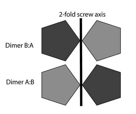
Often, there's more than one way to interpret a centering peak. They can, of course, just be treated as purely translational symmetries. This is a valid way of looking at them. Often, however, their true origin is something like a 2-fold dimer NCS axis parallel to a 2-fold crystallographic axis. Consider the following:
The dark and gray pentagons form a dimer whose intra-dimer axis is aligned with a crystallographic 2-fold screw axis. The dark gray pentagons are crystallographically related to each other, and the light gray ones similarly. If the dark gray molecule/pentagon is the "same" as the light gray molecule/pentagon then the top left molecule looks the same as the lower left molecule, and it is pointing in the same direction. There will be a large pseudo-centering peak in the Patterson corresponding to the vector between the two molecules, because all the atoms in the top left molecule have the same vector difference from their equivalents in the lower left molecule.
In this specific case, it's fairly easy to show that a NCS proper 2-fold axis parallel to a 2-fold 2-fold-screw axis will generate a peak on the Harker section perpendicular to that two-fold (e.g. v=0.5 in a P21 Patterson, v=0 in P2). There are fairly obvious relationships between the location of the axis and the location of the Patterson peak (e.g. in the P21 case a point on the axis would be at x=u/2, y=arbitrary, z=w/2 for a pseudo-centering peak at u,v,w). Note that the dimer axis does not have to lie on the crystallographic symmetry axis, merely be parallel with it.
Obviously, you use the best mask you can get, because the better the mask is, the better the averaging will perform. The Uppsala program MAMA will generate a mask from a coordinate file, which might correspond to one or more atoms all the way up to a refined structure. The CCP4 program MAPMASK can be used to define an NCS mask from a correlation map (i.e. the output from MAPROT in correlation mode) which can define a mask based on regions of high correlation with a supplied NCS operator. The program MAMA2CCP4 can interconvert between Uppsala-style masks and CCP4-style masks. Lastly, the hard-core purists can hand-edit their Uppsala-style masks within O, or manipulate multiple masks within MAMA.
With all masks, one has to be careful of not assigning the next protomer's mask in the current one. This tends to cause problems with averaging. Some programs automatically check for this, but it pays to take care with defining the mask to avoid this problem in the first place. There tend to be edge effects in averaged maps at protomer-protomer boundaries because of this issue.
Example MAMA mask creation around atoms from a PDB file. Note that the unit cell and grid must match that of the map you intend to average.
#!/bin/csh -f
#
#   Make a mask around atoms contained with the PDB file "mask.pdb"
#
lx_mama << EOF
new cell 94.952  116.561  109.560   90.000  114.353   90.000
new grid 56 72 68
new radius 6.
new ?
new pdb m1 mask.pdb
!
list m1
!
expand m1
fill m1
contract m1
island m1
!
list m1
!
write m1 mask.mask
quit
EOF
#!/bin/csh -f
#
#   Automatic local 6D improvement of NCS operator
#
lx_imp << EOF
fourier.ccp4
mask.mask
p21.sym
rt_c0.o
Automatic
1.
0.05
2.
0.1
0.01
0.0001
3
Proper
Complete
Quit
rt_improved.o
EOF
#!/bin/csh -f
#
##  AVE : average and expand back into both masks
#
lx_ave -b << EOF
Average
fourier.ccp4
mask.mask
averaged_x2.ccp4
p21.sym
rt_unit.o
rt_x2.o

EOF
Irrespective of actual correlation coefficients, what you're looking for is increased interpretability of the maps, or disordered loop regions becoming more visible, or.... basically anything that is of use to you. Compare the unaveraged map to the averaged map to see what/if/where the maps are better and where they are worse. The worse regions could be excluded from the mask, but where the maps are better go ahead and improve the model in these regions.
This technique is used extensively in virus crystallography to generate high quality averaged maps from really quite crude initial models, in the absence of experimental phase information. However in these cases their intial NCS operations are quite precisely defined.
One approach to maximize the usefulness of averaging in this case, while taking into account this flexibility, is to use different masks for different parts of the structure. Implementation of this is fairly straightforward. One defines a series of non-overlapping "domain" masks, and a set of NCS operators that map each domain mask to it's respective location on each different protomer. One then averages the map within each mask separately in the conventional way using AVE. Areas outside the masks are set to zero, so the multiple locally-averaged maps can then be added together to generate the multiple mask averaged map (e.g. with the program COMDEM).
The utility of multi-crystal averaging depends not just on the degree of non-crystallographic symmetry it represents but also on the extent to which the different maps are useful. Averaging between isomorphous datasets in the same crystal form is redundant since the maps will appear essentially identical before you start. Averaging with garbage maps in different crystal forms will just degrade the averaged map. Again, monitoring the correlation coefficients of the averaging process, and careful consideration of the averaged map is the only way to assess if things have actually got better.
The rt_j1a_to_j3a.o NCS operator that describes the relationship between two non-isomorphous datasets of the same crystal form looks like:
 .LSQ_RT_NCS6D R 12 (3f15.6)
       0.999995      -0.000683       0.003017
       0.000685       1.000000      -0.000615
      -0.003017       0.000617       0.999995
       0.462049       1.271910      -0.295740
and as expected it is nearly unity between datasets in the same crystal form, but with some shift reflecting the non-isomorphism between
these data.
NCS improvement within the same dataset is done in the same way as with intra-crystal averaging, with IMP. However between different datasets you need to use MAVE instead of IMP to do the NCS operator optimization between the two reference frames:
#
# Reference=jong1a Target=jong1c
#
/usr/local/Uppsala/rave_osx/osx_mave MAPSIZE 9000000 << EOF
Improve
jong3a_eden_400.ccp4
model.mask
rt_j1a_to_j3a.o
c2.sym
c2.sym
jong1a_eden_400.ccp4
Automatic
.5
.02
.5
.05
.01
.0001
1
Quit
rt_j1a_to_j3a.o
EOF
#
#!/bin/csh -f
#
# Multi-xtal Average
#
# Reference=jong1a, Targets=jong1c,jong1e,jong3a
#
# Mave does internal averaging and map transformation into reference
# Comap does averaging of multiple maps within reference
#
#
##
## For this first step (j1a in j1a) I imagine you could use AVE, but for
## consistency I use MAVE in the same way as other runs.
##
#
/usr/local/Uppsala/rave_osx/osx_mave MAPSIZE 9000000 << EOF
Average
jong1a_eden_400.ccp4
model.mask
rt_unit.o
c2.sym
rt_unit.o
rt_j1a_A_onto_B.o

jong1a_eden_400.ccp4
jong1a_averaged_in_jong1a.ccp4
EOF
#
/usr/local/Uppsala/rave_osx/osx_mave MAPSIZE 9000000 << EOF
Average
jong1c_eden_400.ccp4
model.mask
rt_j1a_to_j1c.o
c2.sym
rt_unit.o
rt_j1c_A_onto_B.o

jong1a_eden_400.ccp4
jong1c_averaged_in_jong1a.ccp4
EOF
#
#
/usr/local/Uppsala/rave_osx/osx_mave MAPSIZE 9000000 << EOF
Average
jong1e_eden_400.ccp4
model.mask
rt_j1a_to_j1e.o
c2.sym
rt_unit.o
rt_j1e_A_onto_B.o

jong1a_eden_400.ccp4
jong1e_averaged_in_jong1a.ccp4
EOF
#
#
/usr/local/Uppsala/rave_osx/osx_mave MAPSIZE 9000000 << EOF
Average
jong3a_eden_400.ccp4
model.mask
rt_j1a_to_j3a.o
c2.sym
rt_unit.o
rt_j3a_A_onto_B.o

jong1a_eden_400.ccp4
jong3a_averaged_in_jong1a.ccp4
EOF
#
##
## Take each of the internally-averaged maps now all in the same
## jong1a reference frame and add them together to produce
## the final multi-xtal averaged map using COMAP
##
#
/usr/local/Uppsala/rave_osx/osx_comap MAPSIZE 9000000 << EOF
jong1a_averaged_in_jong1a.ccp4
1.
jong1c_averaged_in_jong1a.ccp4
1.
jong1e_averaged_in_jong1a.ccp4
1.
jong3a_averaged_in_jong1a.ccp4
1.

mxa_averaged.ccp4
EOF