Using HKL3000R for Data Collection at Princeton University

Historical Note and Caveat Emptor

We first started using HKL3000 to drive the data collection part of the system after an upgrade to the RAXIS-IV++ controller in 2012. The initial quality of that software was relatively poor with several functional bugs including one or two dangerous ones. The very first version of this document was an extended rant on the theme of how it was unwise that the vendor ship me that pile of junk, and how equally unwise it was of the author (author name still redacted) to regard it as functional.

Nevertheless HKL3000R did improve to the point where it was functional to collect data on the old single axis RuH3R/RAXIS-IV++, or at least if you didn't put too much faith in the strategy program(s). The penultimate version of the RuH3R/RAXIS HKL3000R document is preserved for posterity. This version refers only to the newer version that drives the 007HF/AFC11/Pilatus 300K system. Parts of the original rant may slip through the edit, or there may be new reasons to rant.

Hardware Note

More extensive notes on the hardware are at Xray-Rigaku-007HF-Pilatus-300K.html.

Controlling the Machine

HKL3000R effectively controls the goniostat and detector, indexes data, calculates strategy and processes the data. In both Windows and Linux contexts the XGControl program controls the generator including start/stop and power ramping. The name of the control computer is mol-xray3. It does not have other user accounts other than those used for data collection. It does not have the ability to do "remote" data collection although remote monitoring of the data is on my To Do list.

Comparison with HKL2000

What's Changed Compared to the RAXIS IV++ System

• There are more axes on the goniostat - use Collect>Align to move the goniostat into Crystal Mount position via the button of the same name or to Zero Goniostat a position with all axes at zero degrees. Use Collect>Manual to move the goniostat to some other position manually.
• There's a video camera - see it in Collect>Align, but note that this is not a "click to center" arrangement and you must still adjust the goniostat.
• Rigaku Strategy program - present in the previous version, using it is now essential since there's more than one axis to consider.
• Smaller detector means that you're more likely to use the Multi-Run Data Collection in the Collect Tab (press the Multi button). For single runs you might need to specify the φ and χ values in the fields on the Collect>Collect tab.

Other Manuals

• HKL2000 manual from HKL Research
• HKL3000 manual from HKL Research as a PDF - doesn't deal with machine control and data processing in any significant way.
• Daniel Gewirth's older Denzo/Scalepack manual is sometimes more useful in that it discusses more of the nuts and bolts of these two programs, which are still the ones doing data processing in HKL2000 and HKL3000, but this older manual is now a decade out of date so some of the recent updates in scaling are not reflected in it.
• HKL2000 manual from SSRL.
• HKL2000 at SER-CAT (APS).

TL;DR - a quick outline of workflow

1. Initiate communication with device using Connect button in Collect tab
2. Goniostat in mount position (Collect>Align); mount crystal and center
3. Test shots at 0° and +89° for 10 or 30 seconds per 0.25°
4. If OK then index using Index tab, select primitive triclinic in Bravais Lattice
5. Refine as Fit Basic and Fit All then click Bravais Lattice to select likely correct lattice (symmetry)
6. Refine with Fit All and then mosaicity
7. In Strategy tab first select space group (if known) then launch Rigaku Strategy, edit to taste, exit strategy and Load DC to put strategy in Collect tab
8. Start data collection via Collect Tab
9. Check integration parameters (spot size, profile fitting radius etc), start integrating data runs
10. Scale data to check for quality and potential point groups
11. Finalize scaling (Error Scale Factor to change χ²), educated guess on space group
12. Close program, go have celebratory beer

Using the Graphical User Interface (HKL3000R)

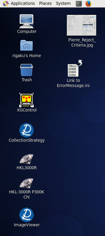
	The computer is always left running, usually logged in, usually running the Linux side of the dual-boot setup. Upon login, the default Desktop has icons for the software on the left-hand side. There are two gaudy diamond icons on the left labeled "HKL3000R" and "HKL-3000R P300K Chi". You want to use the HKL-3000R P300K Chi to control the machine. The HKL3000R version of the program can be used to analyse data you've already collected and cannot control the machine. Other icons of interest are XGControl for controlling the generator, ImageViewer which is apparently Rigaku's image viewing program, and a standalone version of the Rigaku Strategy program - probably not a lot of use without importing Denzo's idea of crystal and goniostat parameters. On the top of the window is the icon bar which you can use to open a Terminal if you want to use standard Unix commands (e.g. for looking in your home directory or managing data). That's the icon right next to the System menu. The web browser (Firefox) is the icon next to that. Since this is a data collection/processing machine, do not install any additional software on this system without permission. CCP4, SHELX, HKL2MAP, XDS are already installed if you want to do other calculations. Other programs (e.g. Phenix) are likely to be added in the near future.
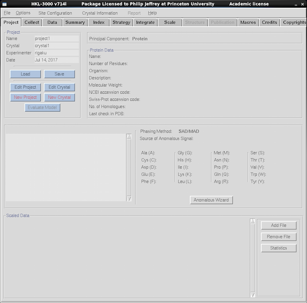
	Quit any existing instances of HKL3000R to avoid accidentally overwrite other people's data. Start the software by clicking on the HKL-3000R P300K Chi icon. Underneath the top menu bar is a series of tabs labeled Project, Collect, Data, Summary, Index, etc. Click on each tab to reach the function for each. If you're screening crystals you'll just use Project and Collect. If you're collecting data or want to auto-index your data you will use more of the tabs further to the right. If you've used HKL2000 then the general layout is familiar. HKL2000 is a data processing program that uses the underlying programs Denzo and Scalepack, and HKL3000R is an extension of that program to control the machine as well as process the data. Use the Project and Crystal framework to keep images for each protein under a distinct project name, with different crystals being a new crystal within a project. Avoid making names absurdly long. Click on the Project Tab to manage projects and samples (shown at left). You can create new projects, save existing ones, load old ones. When HKL3000 starts it defaults to a generic project name - it doesn't save your old project info so you should remember to save it manually before quitting and load it after starting. It's possible to collect data and process it without changing the default project name. Just make sure you specify a separate and unique data directory name for your data and processing directories. I generally recommend against doing this if you're actually collecting data since it makes more sense to cluster related datasets into one project. Also, NEVER modify someone else's project in this way. To reload an existing project, use the Load button within the Project tab and locate the relevant .sav file in the /data directory (scroll past the subdirectory names to find them). An alternative to this interface is to use the Project, Crystal and Base Directory fields in the Collect tab. In all cases the data filenames are /data/Project_Crystal/Project_Crystal_0000.img where Project and Crystal are taken from the values that you've given. The "0000" gets automatically incremented, starting at 1, when you collect images. You can use the Data Directory field in the Collect tab to provide a different directory structure (e.g. grouped by name, lab etc).
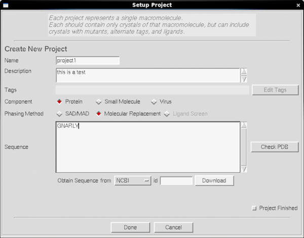
	Here's what you see if you click on the New Project button. Because HKL3000 has tries hard to be an overall framework for structure solution, it can be more pedantic about projects than the old CrystalClear software - however you don't need to give it the sequence for project/crystal and can leave it blank. The main reason to enter it is if you plan on using HKL3000R to solve your structurefor you (not covered here) where the sequence is useful for finding homologs or calculating the expected number of sulphurs. You can solve Hen Egg-white Lysozyme using S-SAD from good tetragonal HEWL crystals, but your crystal probably doesn't diffract like chicken Lysozyme and when I try and do that party trick I do it on my own desktop iMac using HKL2MAP or CCP4i - both of those are available on mol-xray3 too. Most of the options on the project screen are a waste of time for the simple purpose of crystal screening. Nevertheless it's a good idea to use New Project and New Crystal to manage subdirectories and filenames - or the equivalent fields in the Collect tab - since the facility manager is very likely to delete generic "project1" files if the disk starts to fill up.
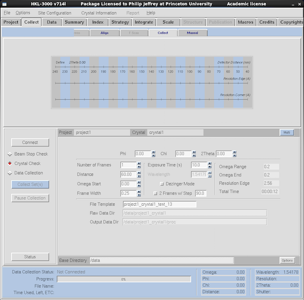
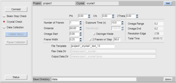
	The Collect is by far the most important tab. To start doing something productive you should mount your crystal and click on the Collect Tab which brings up what you see at left. The buttons on the left are the important ones. You need to press the Connect button to get the program to talk to the machine - this establishes connections to the servers in the generator itself. It also initializes the detector and all axes on the goniostat when it does so - this takes a while since the goniostat isn't all that fast. LOCK DOWN THE PHI (φ) AXIS BEFORE CLICKING ON CONNECT. Below the Connect button the radio buttons select what type of experiment you're doing. Crystal Check loads default parameters for the sort of images we shoot to test crystals. Data Collection are the sort of parameters you'd use if you actually want to collect an entire dataset. We'll come back to those settings, below. Make sure you define a Project and Crystal either via the fields in this tab or via the Project tab. The screen shot at left is from the Collect sub-tab within the Collect tab (yes, that's confusing) but there are two other tabs within Collect that are useful: Align and Manual.
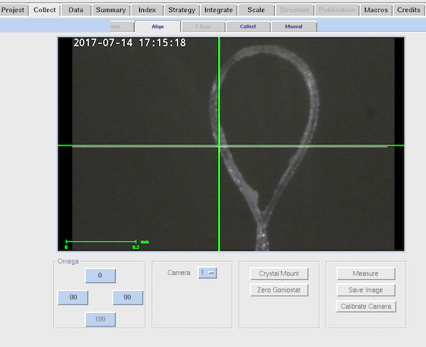
	This is the Align tab within Collect. Since the new system has a video camera for crystal centering you can easily check on crystal status without getting anywhere near it during exposure. You cannot adjust the centering from here. The most useful part of the Align sub-tab is the Crystal Mount option that drives the goniostat to the appropriate position to mount and remove your crystal. You can also drive to ω=0, φ=0, χ=0, 2θ=0 and distance=100 using the "Zero Goniostat" button. Loosen the grub screw on the phi axis to mount your crystal. When centering your crystal be aware that for best results you need to point a translation sled toward the camera and not toward you. The camera is 30° away from the collimator axis (i.e. to front left from the user point of view). You want to adjust the sled that is perpendicular to the camera. Takes a little while to adjust to if you're used to the former optical microscope being right in front of you. If the crystal is moving weirdly on centering check that you're doing this. The goniostat has no vertical adjustment on the phi axis, but there is a certain amount of vertical travel on the goniometer head. Be sure to mount your (empty) loop before starting the experiment to make sure the height is approximately correct and your pin length will work on this setup. The standard length of 21mm (sometimes called 18mm pin length) will work just fine. Remember to tighten the grub screw on the phi axis once your crystal is centered.
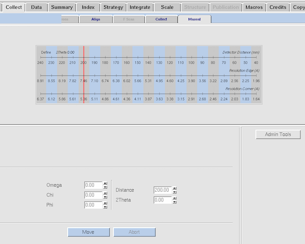
	This is the Manual tab within Collect. If you want to drive to a specific goniostat value, this is where you'd enter it. Most of the time "Zero Goniostat" and "Crystal Mount" within the Align tab would do the job. The current limits on goniostat angles are: 2θ=+5 to -90°; φ= unrestricted; χ= 0 to +45°. The ω axis limits are correlated with the 2θ position (potential collisions between the χ track and the detector) - any angle where the χ axis forms an acute angle with the 2θ track are excluded - but angles around ω=zero° are always collision-free. Generally speaking be ultra-cautious about driving the goniostat into positions manually - drive them perhaps half-way and visually check for potential collisions. The internal software checks should prevent user-generated SNAFUs.
	Now, back to the Collect sub-tab within Collect. Below the Connect button the radio buttons select what type of experiment you're doing. Crystal Check loads default parameters for the sort of images we shoot to test crystals. Data Collection loads the sort of parameters you'd use if you actually want to collect an entire dataset. For Crystal Check you should set distance, number of frames, omega (ω) start, frame width (0.25° perhaps - err on the side of smaller images with the Pilatus, but not <<1/3 of the mosaicity), exposure time (10 seconds is a good start) and click the toggle if you want to shoot orthogonal pairs of images separated by 90 degrees. Limitations of the goniostat mean that sometimes it's better to separate them by 80° or perhaps -90° since at 2&theta=0° an ω=+90° is in the forbidden range but ω=89° or ω=80° is acceptable. Once you've changed the values the blue button at left marked Collect Sets will be enabled and you can collect the images. The new system is quite fast - moving the goniostat is one of the slower steps but typical exposure times are short (seconds) and readout is very fast (milliseconds). With the old single axis goniostat on the RAXIS system, the rotation axis was called phi (φ). Note that with the multi-circle goniostat the scan axis is always omega (ω) rather than phi - this is typical of multi-axis of goniostats where ω is the more accurate axis used for scanning and the axes χ and φ are used for repositioning only. For actual data collection use the Data Collection button which has many of the same parameters as Crystal Check. The current frame is now displayed using the QT version of XDISP (it used to be dtdisplay from Pflugrath's D*Trek) - where the contrast and image zoom are the only significant features. This has a different GUI behavior than HKL's X-windows based XDISP program and runs independently of it. With the smaller detector and a more vesatile goniostat it's likely that you'll be collecting data with multiple runs - in fact you'll probably get better data if you collect with two different φ/χ combinations rather than just one. I'll discuss strategy below - you might have noticed the "Multi" button above-right on the panel and that's where you define the multi-run data collection strategy. Additional features on this tab are: "Status" button at the lower left is the most useful - HKL3000 often rather mediocre notification of what the machine is doing - I've seen it incorrectly report what frame it's collecting. The Status button is sometimes a more reliable source of information.

Most of the steps in data processing are analogous to my HKL Data Processing Guide which was written in 2002, prior to the era in which y'all have been reduced to button clicking for a living. The basic programs in HKL still underlie how HKL2000 and HKL3000 work - they just write scripts to run these programs via the command line and parse the log files. Since I'm both a Luddite and a Curmudgeon you'll frequently find me muttering while reading the actual logs rather than the pretty little graphs.

Strategy Considerations

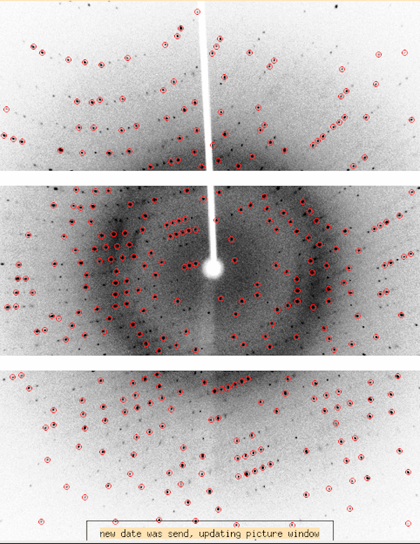
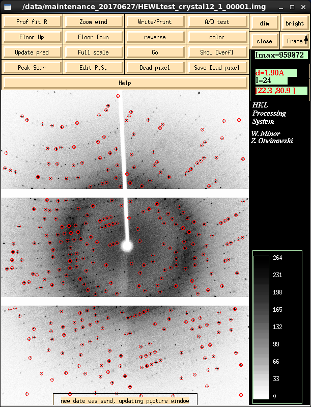
The Dectris Pilatus3 R 300K detector (P300K) is a smaller detector (84x106mm2) than the RAXIS-IV++ (300x300mm2) and is made of three modules stacked vertically. The image at left is from the XDISP display program. The rotation axis on the home source is vertical (i.e. ω). The smaller detector size in the instance of high resolution diffraction may require you to collect multiple runs of data to cover both low resolution and high resolution data, however for many situations you could collect a medium-resolution data set without offsetting the detector very much in 2θ. This particular example is from definitive Hen Egg-white Lysozyme data (tetragonal form) at 2θ=0° and a distance of 45mm. It's usable to 1.9Å without offsetting 2θ and has exceptional merging statistics. Tetragonal HEWL has a max cell dimension of 79Å and we could have collected a little closer. Desired maximum resolution, point group symmetry and the largest primitive cell dimension of your crystal all come into play with strategy. The closest distance for a largest unit cell dimension of A is A/2 with the closest distance between crystal and detector being 34mm. This is better than the RAXIS-IV which was A/1.5. As far as I know the neither the HKL3K nor Rigaku Strategy program estimates the maximum resolution from the test images you have collected - so you still have to eyeball it based on the images you have taken (and/or data you have integrated and scaled). I recommend adding 0.2Å to whatever it is you can see visually because the detector has a habit of pleasant surprising you - and because you can always reduce the resolution limit during processing, but you can't incorporate data you didn't actually correct Usually optimal data collection strategy is where the highest symmetry axis of the crystal is almost parallel to the rotation axis. However with the module boundaries being horizontal - perpendicular to the rotation axis - this might give rise to systematic discs of missing data - and this is likely to be more pronounced in low symmetry space groups at lower resolutions. You might have to incline the symmetry axis more, and this is where the strategy program comes in, and where the partial 4-axis goniostat is of assistance. Collecting data at more than one distinct crystal orientation (φ, χ) is likely going to improve your actual data quality anyway.

Indexing and Generating a Strategy

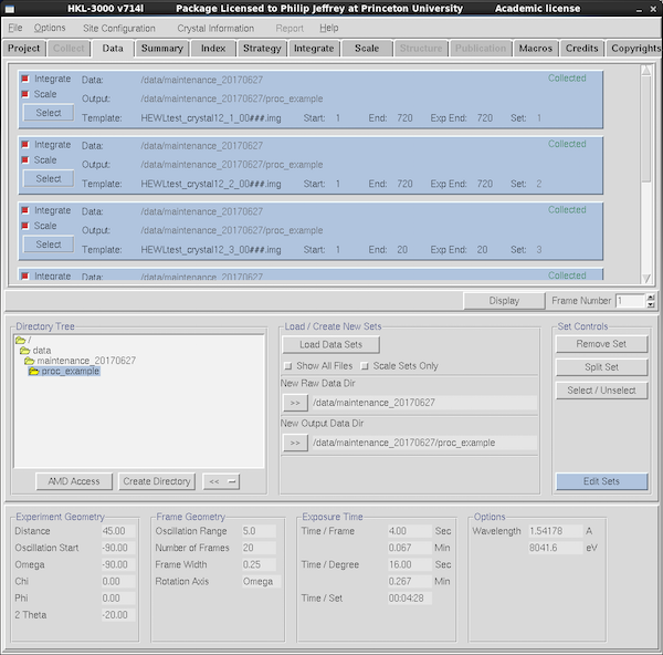
	In the Data tab HKL3000 will load all data runs associated with the project - both test images and data collection runs, and also for data runs that are about to be collected. The blue boxes mark the individual blocks of data. To remove irrelevant data runs, press Select in the blue box and then Remove Set in the Set Controls panel. The red check buttons within each blue data run block offer control whether the data is scheduled to be integrated and scaled. For initial indexing you need only one frame from one data run so perhaps deselect the others - in particular the Project/Crystal framework will often populate the Data window with data from all samples for that project. Also when processing data after collecting test oscillations, make sure you deselect those test frames since they add nothing to the data. If the data directory doesn't show up automatically, navigate to it via the Directory Tree navigation panel at center-left, click to select the directory and press the >> button next to New Raw Data Dir. Select the processing subdirectory similarly and/or create your own. Data collection parameters for the selected data set are shown at the bottom of the tab. To change the expected number of frames in a data set, select it using the SELECT button, and click the EDIT SETS button (center-right). Normally the correct number is found automatically, but you can use this to exclude ranges of frames at the start or end of a set from processing.
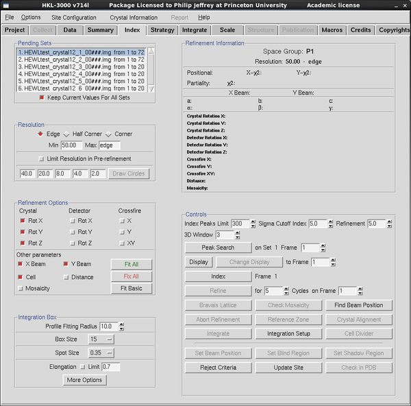
	Indexing your diffraction pattern is a necessary precursor to strategy calculation - symmetry axis orientations need to be known. Go to the Index tab - verify that the data frame(s) listed are the ones you want to index via the panel at top left - adjust via the Data Tab. The text panel at top-right will contain the information for indexed/refined unit cell parameters etc. The buttons below-right control the workflow within Index. The check boxes below-left control what parameters you want to refine to improve predicted and observed spot positions, and a few things about spot size. Click the DISPLAY button to view any frame within the run selected at top left. Click PEAK SEARCH to pick spots on the frame. Unlike XDS and MOSFLM, Denzo auto-indexes from a single frame. Most of the time this works, but potentially less precise than extracting the information from a pair (or range) or orthogonal images.
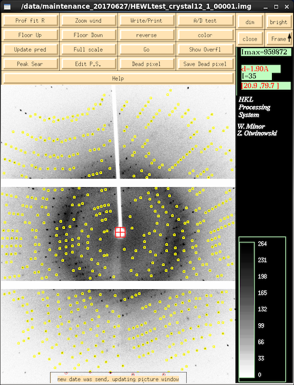
	Denzo's graphical component - XDISP - is shown on the left in peak search mode where it has searched for diffraction maxima based on default criteria. These work well with strong diffractors. With weaker diffractors and troublesome auto-indexing situations you want to click on the Peak Sear button and pick more or less reflections than the default. You can also do Peak Search on images that are not the first one in the data run, by entering the frame number in the box next to the peak search button. For really problematic indexings I try every 10th frame to get an indexing that I believe to be correct and work from there. Denzo is smart enough to take into account the offset between frame N and frame 1 when integrating the data. It is possible to add spots from more than one contiguous set of images. But you can't do it via the Peak Search button in HKL3000. First, use DISPLAY to bring up the first image in XDISP. Press the Peak Sear button in XDISP itself (lower left in button stack). Then middle-mouse click on the Frame button at top right in XDISP to load the next image, which will also peak search and the peaks added to the list. Repeat for a few more frames. This way, the peaks will be accumulated off multiple frames - and it also appears to improve the mosaicity estimate during initial auto-indexing. Once you've got enough data spots selected - and sometimes I select an abundance of spots on the frame and let Denzo sort out the wheat from the chaff - press the INDEX button in the Index tab.

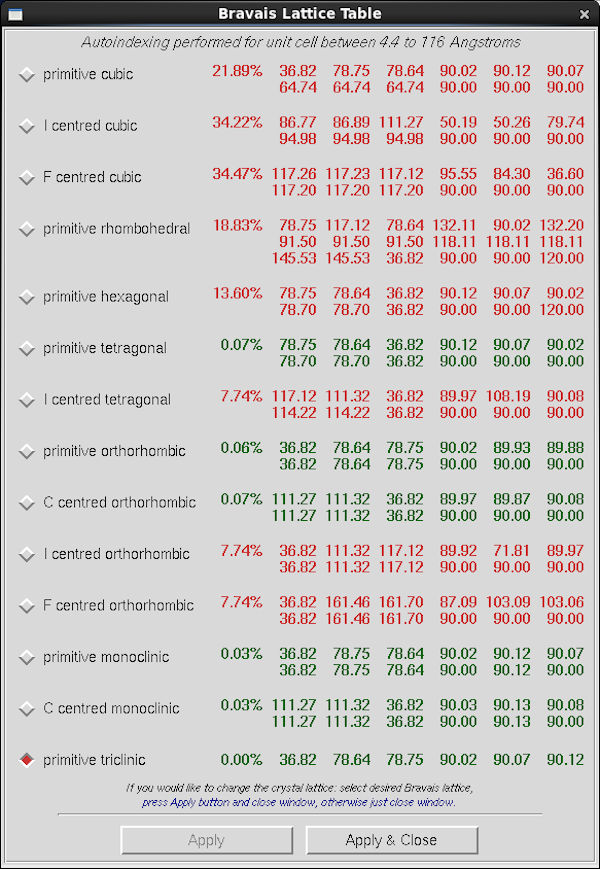
	Denzo presents this table of possible indexings in the "Bravais Lattice Table". The first one to pay attention to is primitive triclinic all the way at the bottom - this is the inherent spot arrangement on the frame and the largest value here corresponds to your smallest inter-spot spacing. It's a Primitive (P) unit cell which means that there aren't any of the systematic absences present in C,F,I lattices that lead to a large proportion of the reflections being systematically absent. On the lines above primitive triclinic, Denzo permutes and potentially distorts that unit cell to obey the symmetry-mandated requirements for each subsequent Bravais lattice, with highest symmetry toward the top. The percentage value it the degree of distortion required. Values in green required relatively little distortion and those in red require more distortion and are unlikely to be correct. Of the pairs of cell dimensions the top one is the permuted cell and the bottom one is that cell after it's "clamped" to the symmetry requirements. For primitive tetragonal, which is what this unit cell is, the requirements are a=b and α=β=γ=90°. For weak auto-indexing results it's best to refine the auto-indexing result in primitive triclinic first and then re-open this table using the Bravais Lattice button in the Index tab. Success can be influenced by the parameters for Index Peaks Limit and Sigma Cutoff Index in the first line of the Controls panel within Index. Be aware that the Bravais lattice table is responding only to the location of diffraction spots in the frame and not their intensity. While the highest symmetry choice is often the best one - for HEWL the point group is 422 with a primitive lattice so primitive tetragonal is indeed the correct choice - a minority of crystals show pseudo-symmetry and the correct assignment of point group and unit cell dimensions only becomes obvious during scaling. At which point you must revisit the Bravais Lattice table and re-integrate the data. To refine the initial indexing result (e.g. in Primitive Triclinic) you select Fit Basic, refine a few times, then Fit All refine a few times more and then revisit the Bravais Lattice table for your best guess at the actual crystal symmetry/lattice system.
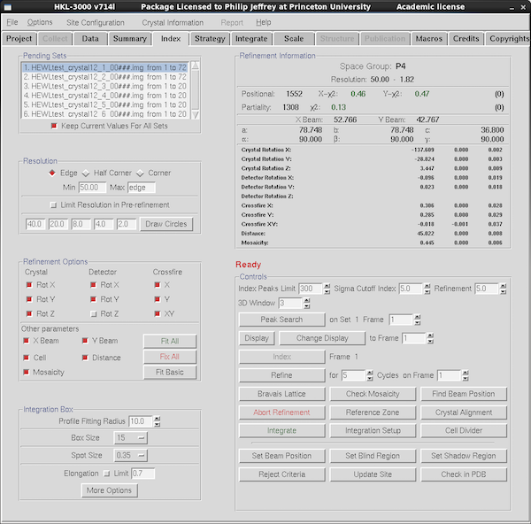
	The current parameters are shown in the Refinement Information panel at top right. For integration you basically only need to produce a good correlation between predicted and observed diffraction maxima - some changes in Bravais lattice can be accommodated in scaling even if you've integrated it as the lowest symmetry primitive triclinic. However it often stabilizes refinement to have the correct Bravais lattice assigned, and it avoids you having to think about complicated transformations (and applying them) in Scalepack later on. To optimize the predicted vs observed maxima you need to refine the initial auto-indexing parameters. The boxes toggled in the Refinement Options panel at the left show what parameters are are being refined the next time you press the Refine button. Some eigenvalue-filtering hopes to reduce the correlations between parameters but the idea here is to Fit Basic until convergence, add in Distance and perhaps Fit All with mosaicity unchecked, followed by Fit Basic with mosaicity checked, followed by Fit All again. Mosaicity estimates are sometimes problematic for crystals with streaky spots, and if the refined mosaicity climbs too high it will likely cause problems with spot overlaps (spots whose centroids are too close to each other on the frame). You can play games with not refining mosaicity or you can redefine it at each integration step using the Macros tab (not covered in this guide). For weak data you'd probably do well to decrease the sigma cutoff for data in refinement, as given in the Refinement box in the Control panel to the right. If you're unhappy with the spot predictions and wish to discard the current parameters you'll need to press the Abort Refinement button to go back and do peak searching or indexing again.
	Once you've started refining parameters, XDISP changes to display the predictions of spot centroids based on the refined parameter values - toggle this using the Update Pred button to see if the predictions (yellow, green, red) match the actual spot locations. Yellow centroid markers are partial reflections - reflections that are clipped at one or both ends of their profile during the frame and whose diffraction intensity is spread over multiple frames. Green reflections are full reflections that complete their entire passage through diffraction condition during the frame. On this image - collected with 0.25° frame width on a crystal with 0.45° mosaicity - every reflection is a partial. You only see a significant number of fulls on thicker frames, particularly at higher resolutions. Reflections with centroids that are red have issues - highly variable background, overloads (unlikely with this detector), spots that are too close to each other ("overlaps").

If the predicted spot centroids match the observed ones well enough you can then move to the next tab - Strategy - to calculate the runs necessary to collect a complete data set. Again, you'll have to use existing images to assess the likely limit of diffraction based on your current exposure time, although of course you can adjust this during the data processing step.

Strategy

After auto-indexing, click on the Strategy tab and change the space group as necessary - inherently you're making a decision on point group rather than actual space group at this stage. By default Denzo will opt for the lowest-symmetry space group/point group within the Bravais Lattice that you selected. In this case it's space group P4 in point group 4 (Laue group 4/m). Tetragonal lysozyme is actually space group P4₃2₁2 in point group 422 (Laue 4/mmm) which affects the strategy since 422 is higher symmetry than 4. If you don't know what your space group is, stick to the default. The worst that can happen is that you'll collect more data than you need.

Click Rigaku Strategy to launch the program. Click Yes I Want To Make Changes. In the sidebar are options for completeness (recommend: 98% or greater), redundancy (recommend: 3 or greater), resolution (you'll have to eye-ball that) etc. Click Calculate Strategy to get the program to come up with something.

Data Processing

Denzo will pick up goniostat values from the frame header, so if your crystal remains in the same position on the goniometer head during the different runs you should be able to use the same relative indexing - this is particularly important in point groups 3, 32, 4, 6 to avoid the relative indexing problem (see CCP4's reindexing page). This would show up in scaling but understanding why it happens is very useful, particularly when comparing multiple crystals.

Go back to the Data tab and select the runs you want to include in data processing, likely excluding the test images you took when assessing data quality or assessing a strategy. Index the data and refine the parameters using the Index Tab in exactly the same way I outlined above.

Check again the correspondence between predicted and observed spot centroids. Yellow and green reflection centroids are partials and fulls, respectively. Red reflections are ones with a problem: overloads (unlikely on the P300K); overlaps (spots that are too close); spots with badly behaved backgrounds (too close to module boundaries etc). If that looks OK be sure to check the spot integration parameter on the lower left of the Index tab under the Integration Box panel. Denzo, like other refinement programs, uses learnt profile fitting to provide a better estimate of weak data by estimating weak spot profiles by generating empirical spot profiles from nearby strong spots. Profile Fitting Radius sometimes needs to be increased for particularly weak or anisotropic data or Denzo will refuse to integrate weak data with insufficent nearby strong spots to estimate the profile from. Historically it also paid attention to one of the sigma cutoffs (perhaps refinement?) shown in the Controls panel - that defined the σ(I) boundary for what was considered strong vs weak. Only strong spots are used to construct spot profiles.

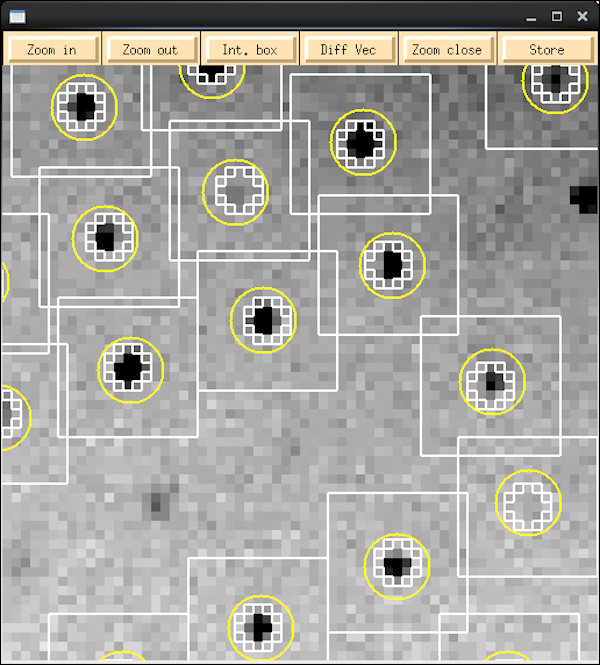
To get a look at the spot size, first click on Zoom Wind button in XDISP to open the zoom window, then middle-mouse click somewhere on the master image to center the view in the zoom window. Click on Zoom In a few times to, well, zoom in. Click on Int Box to show the integration box. The square is the background box that Denzo fits a least-squares plane through to subtract the background from the spot prior to integration. It's OK for those boxes to overlap - that's controlled by the Box Size parameter in the Index tab. The box needs to be several times the size of the spot to get a reliable background estimate. The yellow circles are the spot centroid positions (yellow=partial, same as before) and inside these are two concentric circles around the spot, although it's not that obvious in this image since the spots are only a few pixels wide. The central one is controlled by the Spot Size parameter in the index tab. The point spread function on the P300K is relatively small so spots are usually quite small (and the pixels are larger at 170µm) but it's important that the spot size encompass all of the reflection - increase Spot Size as necessary after sampling various parts on the image. If you change these parameters you have to do one cycle of Refinement to update the view in XDISP. Caution: if you make the spot sizes too large, adjacent spots will overlap each other and Denzo will reject these spots as "overlaps". The spot centroids show up as red in this case. Are we done yet ? If you've got the parameters refined so that the predicted spot centroids match reality, you've selected the correct Bravais lattice, and you've tweaked the spot size parameters as necessary you're pretty much good to start integration. However if your crystal does not diffract to the edge of the detector there's not much point integrating fresh air - you can limit the resolution for integration via the Resolution panel in the top left corner. Conversely if you have really strong data (as this is) you could integrate into the Half-Corner or Corner of the image, although you'd get far better data coverage if you moved the detector closer (if possible) or moved the detector further out in 2θ. You will need to do one cycle of refinement, again, if you change the resolution limits.

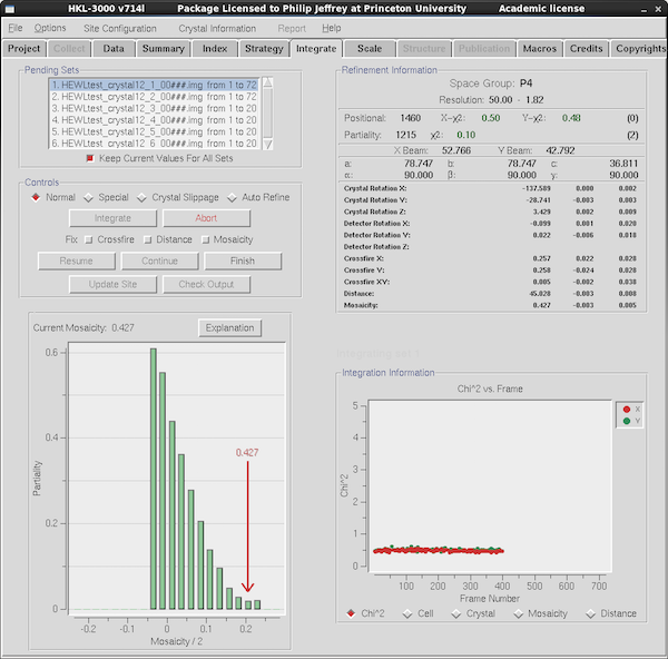
Go to the Integration Tab to start integration. Generally speaking most of the parameters that affect integration are actually on the Index tab. But if you particularly want to fix mosaicity during integration (e.g. for smeared spots or crystals with other types of large mosaicity issues) then this is the place to select it - in the Controls panel at top left. Check that the data runs listed in the table at top left are all the ones you want to integrate, then press Integrate. If this is not the first time you've integrated the data you'll be prompted if you want to overwrite the ".x" files or create a new subdirectory. I nearly always do the former. Denzo writes a file with extension ".x" that contains the spots that are integrated on a particular image, as well as the current integration and crystal parameters. Scalepack then reads all these .x files to scale and merge the data. During integration Denzo will happily wait for frames that are being collected - just make sure it isn't hanging up at the end of data collection waiting for frames that will never arrive. Denzo will display the position residuals (chi2) for detector X and Y between predicted and observed spot positions. Something less than 1.5 is desired here. The "Integration Information" panel at lower right will show you positional chi2, unit cell parameters etc during integration. It's not all that uncommon for one or more parameters to drift during integration since the initial indexing was done of one frame and the parameters are refined locally off one or a very small number of frames - they aren't estimated over a large angular range. Nevertheless you shouldn't see mosaicity or distance wander very much (although mosaicity can be anisotropic). If they do you might consider fixing them during integration. Most of what goes on in the integration tab isn't all that exciting in terms of monitoring data quality, but you still want to make sure those residuals are small.

Scaling

Inherently a number of semi-empirical parameters are refined to minimize the intensity differences between observed reflections that should have the same intensities based on symmetry. This requires an expectation of what the error should be based on the strength of the data and of what the likely point group symmetry is.

Symmetry: in this example we picked a Bravais lattice (i.e. primitive tetragonal) which can accommodate two different point groups, 4 and 422. The former has a single four-fold symmetry axis and the latter also has two-fold symmetry axes perpendicular to the four-fold. Alternatively speaking: point group 4 has eight symmetry-equivalent reflections in a complete sphere of data and 422 has sixteen of them (assuming Friedel's Law holds - no anomalous scattering). By picking a space group that is compatible with the Bravais lattice you intrinsically assign a point group to the data: space group P4₃ is in point group 4 and space group P4₃2₁2 is in point group 422.

Friedel's Law: Friedel's Law applies in the case where anomalous scattering contributions are very small. It introduces a center of symmetry in the data, so that reflections (h,k,l) and (-h,-k,-l) have the same intensity. Elements C, H, N, O have minimal anomalous scattering at CuKα wavelength (1.54Å) but S, I, Lanthanides do not. For some well-diffracting proteins - like the HEWL xtal here - you can actually use the very small sulphur anomalous scattering signal to determine the structure but for weakly diffracting proteins you can mostly ignore the presence of this signal.

Scaling: Scalepack is the program that does the scaling. There are some behind-the-scenes analytical corrections for Lorentz and polarization factors, air absorption etc but then Scalepack refines a per-frame scale factor (k) and a per-frame B-factor (B) as a primary method of reducing systematic differences in the data - i.e. the differences in measured intensities of reflections that should be indentical based on point group symmetry. As k,B are expected to be smoothly varying they are often restrained during scaling. If you turn on absorption correction it will additionally refine an empirical absorption correction parameterized as spherical harmonics. The scaling model is described in Dominika Borek's CCP4 presentation from 2009. The per-frame correction factors model things that vary primarily with image number, of which primary absorption and scattering effects due to the variation of the volume of the crystal in the beam are the main one, and a B-factor term that potentially models the impact of radiation damage on the crystal (fall-off in scattering with respect to resolution). In reality things aren't quite that clean, since anisotropic scattering will turn up in part in the per-frame B-factor, and longer-term variations in e.g. detector response or beam intensity get folded into the per-frame scale factor. An absorption correction that is additional to this "k+B" scaling also serves to reduce errors and is doubtless analogous to the existing methods in XSCALE(XDS)/SCALA/AIMLESS. In any event, all scaling methods involve exploiting the redundancy in your data as a method for estimating the quality of the scaling result is going to improve as the redundancy of your data improves. The estimates of the mean intensity of the unique reflections also improves with increased redundancy.

Quality Estimates: R_merge is a simple statistic that reflects the proportional deviation of reflections that should have the same intensity based on symmetry. Its synonym is R_sym and they are used interchangeably in the modern era. R_merge is systematically under-estimated for data with low redundancy and approaches its "true" value only in the case of high redundancy, which is inevitably a higher R_merge. This presents the ironic situation where low-redundancy R_merges are lower than high-redundancy R_merges for the same data, despite the expectation that the high-redundancy data has better-estimated intensity averages. To deal with this, R_meas was introduced which is the redundancy-compensated version of R_merge (see XDS wiki) and is more reliable over a larger range of multiplicities. See Diederichs & Karplus (1997). Scalepack now reports R_meas as well as R_merge. Both R_meas and R_merge should be in the low single digits for the low resolution (i.e. strongest, best measured) data after scaling and will inevitably rise towards the high resolution cutoff which corresponds to weaker data. R_merge<=R_meas. The useful high resolution cutoff is a matter of active debate but probably data can be considered useful up to R_meas values above 60% and possibly even above 80% but up in these "nose-bleed" ranges the statistic CC_1/2 is more useful. CC_1/2 is the correlation coefficient between data randomly split between two halves of a data set. Current rules-of-thumb suggest that one should include data with CC_1/2 higher than 0.5, although my own experiences suggests that I'm more comfortable with a cutoff that is around CC_1/2 ~ 0.75. Here again, however, CC_1/2 is not going to be accurately estimated if you have no redundancy in your data. (For more on the how-long-is-this-piece-of-string/how-far-does-my-data-go discussion see: Evans & Murshudov (2013) and references therein - the goalposts have been moved but you still have to use your brain and perhaps use the paired refinement technique in order to exploit this weaker data).

Postrefinement: Under the Global Refinement section of the scale tab there's a variety of options that fall under the general heading of postrefinement (so named because it occurs after the data integration step, but "global" is perhaps a more informative name). Recall that during indexing and during integration the refinement of parameters - particularly unit cell dimensions - the refinement is quite local and doesn't consider the whole of diffraction space. Parameter refinement may quite easily fall into false local minima during minimization. Postrefinement - activated if you select anything above the bottom option - considers the location of diffraction maxima on all the frames at once, so in particular it should provide much more accurate unit cell dimensions for downstream use. It also provides more accurate estimates of the Lorentz correction which can be large for low resolution reflects that lie near the rotation axis. Usually you want to do some form of postrefinement even if it's not immediately obvious which of the options is most appropriate (and in anything except pathological cases there is little difference).

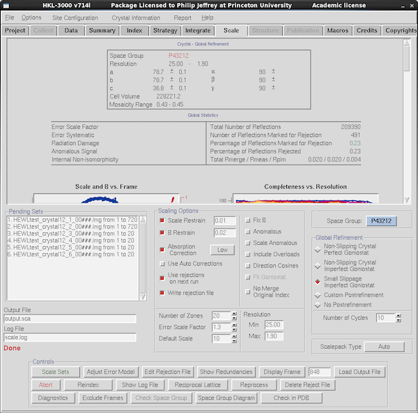
The actual process of scaling is easier to comprehend than the more theoretical discussion above. Select the Scale tab. Make sure the data runs you want to merge are included in the "Pending Sets" list. Click on the toggles for Scale Restrain, B Restrain, Absorption Correction (Low), Write Rejection File and over on the right Small Slippage Imperfect Goniostat. Leave Use Rejections on Next Run unchecked. Pick the low resolution cutoff as 25Å since the beam stop is fairly small on this new system. If you've done any prior scaling click the "Delete Reject File" button and then at the top left of the button array in Controls, click Scale Sets. What you've done is scale all the data runs lumped together, minimizing the discrepancies between symmetry-related reflections. It'll take a few seconds to do this and then the GUI will parse the Scalepack log file and populate the graphs in the upper selection of the scale tab with a summary of the Scalepack log file. You can view the actual file (sometimes easier) using "Show Log File". But the second table from the top - "Global Statistics" - is a pretty good summary: 209K observations with <500 marked for rejection (the green color for 0.23% indicates "this is good") and an R_meas of 2.0% for data in the range 25-1.9Å. This data goes much further but this is the acceptance criterion data set and 2.0Å is all we need for that purpose. By default Index (and therefore Integrate) will select the lowest-symmetry point group consistent with the Bravais lattice you selected in the Index step. Assuming you don't have pseudo-symmetry or twinning this is a good choice for the initial scaling run (which would have been done in P4 in this case) and then you can explore how changing the space group changes the scaling statistics. Changing the point group from 4 to 422 might change them a lot (e.g. from space group P4 to P422) but changing between P4 to P41 will only make a minimal difference - same point group and P41 differs from P4 only by having some (0,0,l) reflections systematically absent. P41 differs from P42 in the pattern of systematic absences and P43 has the same pattern as P41 because they are enantiomporphic space groups where the only difference is the direction of the screw axis. So while chosing space groups be aware that different space group choices within a point group basically have the same scaling statistics. I knew HEWL grew in P43212 so it was easy to select at the start but it would be identical to P41212 and very similar to P4322 in scaling stats - the best way to tell the actual space group is after the scaling step when you (hopefully) solve the structure. Since you can solve the structure via S-SAD using this data I should have clicked on the "Anomalous" button in the middle column so it would output (+h,+k,+l) and (-h,-k,-l) without merging them.

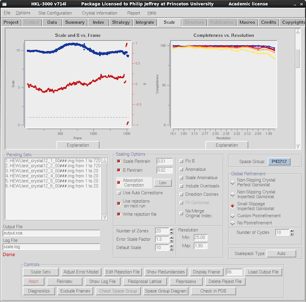
Scroll down in the graphical data tables to see some statistics with resolution or by frame number. At left here is the scale factor and B-factor by frame which you expect to move around smoothly but perhaps jump a little at the boundaries between data runs. Here you can see some disjoint behavior for the last few runs (20 frames each, so 5 degrees) and you might be tempted to omit them from scaling - at the bottom there's a button for Exclude Frames to allow you to omit some especially troublesome frames, but in this case you'd just go back to the Data tab and deselect the Scale checkbox for any runs you want to delete in their entireity. At right is the all-important completeness vs resolution table - if you want to make any real use of your data you want it to be >85% but there's usually little excuse for it being anything <95% unless it's in space group P1. The color-coding is by redundancy (this data is overkill - there's nearly always some separation) and the explanation for the scheme is via the Explanation button, as it is for most graphs.

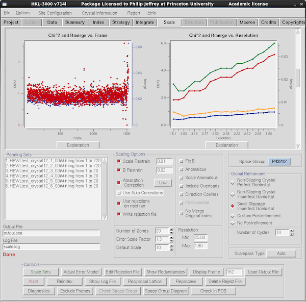
Scroll down some more and you see more data quality tables - here it's R_merge vs resolution and Chi2 vs frame number. Scalepack's error model expects that the Chi2 should be 1.0 for data whose sigmas are estimated correctly. Inherently this is comparing what you'd expect R_merge to be vs what the observed I/σ(I) actually is, and changing the scale of the σ(I) until the Chi2 is 1.0. You do this via the Error Scale Factor just above the button stack - if Chi2 is >1 increase error scale factor by 0.1 at a time until Chi2~1. And reduce Error Scale Factor if Chi2 is <1. You can also adjust the error scales in resolution shells via the Adjust Error Model button. Programs like AIMLESS and XSCALE do all this for you, so here again SCALEPACK is needlessly manual in the adjustments. If you're doing this step you do want to turn on Use rejections on next run to get the best estimate of final scaling statistics, but since this excludes outlier reflections from scaling, and the outlier criteria are based on σ(I) you need to Delete Reject File and do 2-3 cycles of scaling if you change Error Scale Factor significantly. You can get obsessive about adjusting the error model so that Chi2~1 but the most important thing is to get it relatively close. (Ironically modern maximum likelihood refinement programs largely ignore σ(I), although correct σ's are somewhat useful for experimental phasing). The other table is for R_merge vs resolution and, yes, it's using R_merge rather than the preferred R_meas. How very retro. This data is too good to be useful as a discussion point - the R_merge is only 3% in the high resolution bin - and normally you'd see a "ski ramp" with a low % value on the left and your resolution limit on the right, adjusted (the Resolution Max field) so that R_merge is in the 60% range or thereabouts. See the discussion above for "how far does my data go". Best to click Show Log File and look at the last table on the log file to see what CC1/2 and R_meas are in the outermost shell and adjust the resolution cutoff accordingly. The final steps are: adjust your high resolution cutoff; adjust error scale factor to make Chi2~1; check your best-guess for space group; Delete Reject File and do 3-5 cycles of scaling to converge on the final output; go solve your structure.

Downstream Data Wrangling

HKL3000 is not an Expert System